SAS data reduction Haydyn Mertens (EMBL-Hamburg) Data reduction - PowerPoint PPT Presentation
SAS data reduction Haydyn Mertens (EMBL-Hamburg) Data reduction steps Acquisition Reduction Parameters SAXS instrumentation 2D images to 1D profile SAXS invariants - Sample - Integration - Rg - Buffer - Normalisation - I0 (MM) -
SAS data reduction Haydyn Mertens (EMBL-Hamburg)
Data reduction steps Acquisition Reduction Parameters SAXS instrumentation 2D images to 1D profile SAXS invariants - Sample - Integration - Rg - Buffer - Normalisation - I0 (MM) - Background - Averaging/Subtract - Vp
Data Acquisition Detection X-rays, neutrons Detectors
Instrumentation – X-rays • Monochromatic and collimated X-ray radiation • Reduced parasitic scattering • Calibrated detector with low background slits slits primary beam Scattered X-rays beamstop detector Wavelengths ~ 0.06 nm - 0.15 nm 4. December 2017 Haydyn Mertens, EMBO 2017 (Singapore) YEARS I 1974–2014
Instrumentation – X-rays Cf. Al Kikhney (EMBL-Hamburg) 6. December 2017 Haydyn Mertens, EMBO 2017 (Singapore) YEARS I 1974–2014
Instrumentation – Neutrons • Monochromatic and collimated radiation • Reduced parasitic scattering • Calibrated detector with low background Velocity selector collimator collimator primary beam Scattered Neutrons beamstop detector Wavelengths ~ 0.2 nm – 1.0 nm 6. December 2017 Haydyn Mertens, EMBO 2017 (Singapore) YEARS I 1974–2014
The small-angle scattering experiment • X-rays are scattered mostly by electrons • Thermal neutrons are scattered mostly by nuclei • Scattering amplitude from an ensemble of atoms A( s ) is the Fourier transform of the scattering length density distribution in the sample r ( r ) • Experimentally, scattering intensity I( s ) = [A( s )] 2 is measured. k 1 s = k 1 - k 0 =(4πsinθ)/λ k 0 = 2π/λ 2θ Radiation sources: X-ray laboratory λ = 0.1-0.2 nm X-ray synchrotron λ = 0.03-0.35 nm Neutron therm λ = 0.2-1 nm 4. December 2017 Haydyn Mertens, EMBO 2017 (Singapore) YEARS I 1974–2014
The small-angle scattering experiment • 2D pattern collected • Exposure time (ms- sec) • Transmitted beam intensity (beam-stop) • Radially averaged (for isotropic scattering) à 1D profile • Normalisation • Frames checked for radiation damage and averaged • Subtraction of buffer/background 1.0 p(r), rel. units. 0.5 I(s), rel. units. 0.0 0 5 10 15 r, nm 0 1 2 3 4 5 -1 s, nm 5. December 2017 Haydyn Mertens, EMBO 2017 (Singapore) YEARS I 1974–2014
The small-angle scattering experiment • MASKING • S-AXIS calibration • AgBeh (d = 5.38 nm) • Intensity scale calibration • H 2 O 0.0163 cm -1 6. December 2017 Haydyn Mertens, EMBO 2017 (Singapore) YEARS I 1974–2014
SAS sample measurement To obtain scattering from particles of interest: • Subtract scattering from matrix/solvent (also reduces contribution of background, eg. slits & sample holder) Contrast Dr Dr = < r (r) - r s > , where r s is the scattering density of the matrix, may • be very small for biological samples Particle+matrix matrix Difference
What are we really measuring? • Contrast and the other things ... • SAXS intensity profile of “difference” between particle and matrix/background. I ( q ) = ξ d σ ( q ) = ξ n Δ ρ 2 V 2 P ( q ) S ( q ) d Ω Instrument constant Form factor Number of particles Contrast Particle volume Structure factor 4. December 2017 Haydyn Mertens, EMBO 2017 (Singapore) YEARS I 1974–2014
What are we really measuring? • Contrast and the other things ... • SAXS intensity profile of “difference” between particle and matrix/background. Scattering Density I ( q ) = ξ d σ ( q ) = ξ n Δ ρ 2 V 2 P ( q ) S ( q ) Δ ρ d Ω Solute Buffer Instrument constant Form factor Number of particles Contrast Particle volume Structure factor 4. December 2017 Haydyn Mertens, EMBO 2017 (Singapore) YEARS I 1974–2014
What are we really measuring? • SAXS intensity profile of “difference” between particle and matrix/background. I ( q ) = ξ d σ ( q ) = ξ n Δ ρ 2 V 2 P ( q ) S ( q ) d Ω • If dilute enough, S(q) = 1.0 (can neglect) • If n high enough (concentrated sample), we have signal! • If V is big (eg. large protein), strong signal (even if n is small) • P(q) defines the shape • If contrast (Δ ρ = ρ particle – ρ solvent ) is small à see close to nothing! 4. December 2017 Haydyn Mertens, EMBO 2017 (Singapore) YEARS I 1974–2014
Contrast • X-ray scattering densities of solvents and macromolecules Scattering species Scattering density eÅ -3 H 2 O 0.334 D 2 O 0.334 50 % Sucrose in H 2 O 0.40 Protein 0.42 RNA 0.46 DNA 0.55 • Possible to contrast match in an X-ray experiment but tricky! Adapted from Svergun & Feigin, Structure Analysis by Small-Angle X-Ray and Neutron Scattering , Plenum, 1987 4. December 2017 Haydyn Mertens, EMBO 2017 (Singapore) YEARS I 1974–2014
Contrast for X-ray • Matching electron density of sub-complex ( eg. Protein:DNA) I = I DNA + I DNA I PROT + I PROT I = I DNA + I DNA I PROT + I PROT I = I DNA + I DNA I PROT + I PROT Standard buffer (aqueous) ~ 50% sucrose 4. December 2017 Haydyn Mertens, EMBO 2017 (Singapore) YEARS I 1974–2014
Characterise your sample & Look at your data! PAGE/SEC-MALLS/SAXS DATA
D max p ( r )sin( sr ) Standard situation ∫ I ( s ) = 4 π dr sr 0 Monodisperse non-interacting systems Observed scattering proportional to • (averaged over all orientations) Facilitates size, shape internal structure • investigation (at low resolution)
Experimental SAS profile • Form factor of each particle in the solution summed • Monodisperse ideal attractive repulsive • Dilute 4 4 4 2 2 2 0 0 0 0 0.5 1 1.5 2 2.5 3 0 0.5 1 1.5 2 2.5 3 0 0.5 1 1.5 2 2.5 3 -1 -1 -1 s, nm s, nm s, nm
Experimental SAS profile • Form factor and structure factor • Interparticle interference ideal attractive repulsive • Attractive (eg. aggregation) 4 4 4 2 2 2 0 0 0 0 0.5 1 1.5 2 2.5 3 0 0.5 1 1.5 2 2.5 3 0 0.5 1 1.5 2 2.5 3 -1 -1 -1 s, nm s, nm s, nm Inter-particle distances begin to be of the same order as the intra- particle distances.
Experimental SAS profile • Form factor and structure factor • Interparticle interference ideal attractive repulsive • Repulsive (eg. ordering) 4 4 4 2 2 2 0 0 0 0 0.5 1 1.5 2 2.5 3 0 0.5 1 1.5 2 2.5 3 0 0.5 1 1.5 2 2.5 3 -1 -1 -1 s, nm s, nm s, nm Start to see a set of dominant average inter-particle distances (usually only at high conc.).
Parameters from SAS: Radius of gyration R g (Guinier, 1939) 1 Maximum size D max : @ - 2 2 I(s) I( 0 ) exp( R s ) g p(r)=0 for r> D max 3 1.0 p(r), rel. units. D max 0.5 I(s), rel. units. 0.0 0 5 10 15 r, nm Excluded particle volume (Porod, 1952) ¥ ò = p 2 = 2 V 2 I(0)/Q; Q s I ( s ) ds 0 0 1 2 3 4 5 -1 s, nm 4. December 2017 Haydyn Mertens, EMBO 2017 (Singapore) YEARS I 1974–2014
Big vs small objects and the scattering angle! • Intensity drops off more rapidly for larger particles! Δ a = 1λ à all phases uniformly represented 2θ (cancellation of signal) Δ a Δ b = Δ a à signal cancellation at lower angles 2θ Δ b Adapted from: Kratky, O. (1963) Prog. Biophys. Mol. Biol. 13. 4. December 2017 Haydyn Mertens, EMBO 2017 (Singapore) YEARS I 1974–2014
SAMPLE OPTIMISATION ① DATA COLLECTION ② DATA REDUCTION ③ PRIMARY ANALYSIS ④ MODELING ⑤ VALIDATION ⑥ 4. December 2017 Haydyn Mertens, EMBO 2017 (Singapore) YEARS I 1974–2014
SAMPLE OPTIMISATION ① DATA COLLECTION ② DATA REDUCTION ③ PRIMARY ANLAYSIS ④ MODELING ⑤ VALIDATION ⑥ 4. December 2017 Haydyn Mertens, EMBO 2017 (Singapore) YEARS I 1974–2014
Data reduction 1D profiles Averaging/Subtraction Merging YEARS I 1974–2014
Data flow Obtain 1D profiles of frames (sample & buffer) Average frames (in PRIMUS) Subtract background/buffer scattering (in PRIMUS) Guinier analysis Concentration dependent behaviour? No Yes average Merge/extrapolate IFT (eg. GNOM) Fitting (eg. CRYSOL) Modeling 19/06/12 YEARS I 1974–2014
Data reduction: Averaging of frames in PRIMUS lin - lin log - lin Concentration series loaded (including buffers ) 19/06/12 YEARS I 1974–2014
Data reduction Averaging data sets Sample and two buffer sets Sample VS buffer 19/06/12 YEARS I 1974–2014
Data reduction Averaging data sets Average buffers 19/06/12 YEARS I 1974–2014
Data reduction Subtraction of the background (averaged buffer) Subtract average buffer from sample 19/06/12 YEARS I 1974–2014
Radiation damage Frames change Following exposure - Intensity increase - SAS parameters
Concentration dependence!
Concentration dependence • Difference of low and higher concentration data Low conc. High conc. 19/06/12 YEARS I 1974–2014
Merging data sets Low-s region often contains significant structure factor • Option 1: • Use lowest conc data for low-s and merge with high-s from high conc data. • Option 2: • If R g and I(0) change in a linear way with concentration, extrapolate to infinite dilution (remove structure factor) 19/06/12 YEARS I 1974–2014
Option 1: Merging data sets R g changes linearly (or close enough) with concentration 19/06/12 YEARS I 1974–2014
Recommend
More recommend
Explore More Topics
Stay informed with curated content and fresh updates.

