Saddlepoint-Based Bootstrap Inference in Dependent Data Settings - PowerPoint PPT Presentation
Saddlepoint-Based Bootstrap Inference in Dependent Data Settings Alex Trindade Dept. of Mathematics & Statistics, Texas Tech University Rob Paige , Missouri University of Science and Technology Indika Wickramasinghe , Eastern New Mexico
Saddlepoint-Based Bootstrap Inference in Dependent Data Settings Alex Trindade Dept. of Mathematics & Statistics, Texas Tech University Rob Paige , Missouri University of Science and Technology Indika Wickramasinghe , Eastern New Mexico University (former student) Pratheepa Jeganathan , Texas Tech University (current student) June 2014 SPBB Inference Under Dependence ( Dept. of Mathematics & Statistics, Texas Tech University Rob Paige , Missouri June 2014 1 / 21 alex.trindade@ttu.edu
Outline Overview of SPBB inference: Saddlepoint-Based Bootstrap 1 An approximate parametric bootstrap for scalar parameter θ Application 1: Spatial Regression Models 2 Classic application of SPBB Better performance than asymptotic-based CIs Application 2: MA(1) Model 3 Challenging; extend methodology in two directions Extension 1: Non-Monotone QEEs Extension 2: Non-Gaussian QEEs SPBB Inference Under Dependence ( Dept. of Mathematics & Statistics, Texas Tech University Rob Paige , Missouri June 2014 2 / 21 alex.trindade@ttu.edu
Saddlepoint-Based Bootstrap (SPBB) Inference Pioneered by Paige, Trindade, & Fernando (SJS, 2009): SPBB: an approximate percentile parametric bootstrap; replace (slow) MC simulation with (fast) saddlepoint approx (SPA); estimators are roots of QEE ( quadratic estimating equation ); enjoys near exact performance; orders of magnitude faster than bootstrap; may be only alternative to bootstrap if no exact or asymptotic procedures; Idea: relate distribution of root of QEE Ψ ( θ ) to that of estimator ˆ θ ; under normality on data have closed form for MGF of QEE; use to saddlepoint approximate distribution of estimator (PDF or CDF); can pivot CDF to get a CI... numerically! leads to 2nd order accurate CIs, coverage error is O ( n − 1 ) . SPBB Inference Under Dependence ( Dept. of Mathematics & Statistics, Texas Tech University Rob Paige , Missouri June 2014 3 / 21 alex.trindade@ttu.edu
SPBB: An Approximate Parametric Bootstrap Intractable! (And bootstrap too expensive...) θ ( ˆ θ obs ) ( θ L , θ U ) F ˆ pivot ˆ θ solves ˆ θ obs ) ( 0 ) Ψ ( θ ) = 0 F Ψ ( ˆ Ψ ( θ ) monotone SPA via MGF of Ψ ( θ ) θ ( ˆ θ obs ) = F Ψ ( ˆ θ obs ) ( 0 ) F ˆ SPBB Inference Under Dependence ( Dept. of Mathematics & Statistics, Texas Tech University Rob Paige , Missouri June 2014 4 / 21 alex.trindade@ttu.edu
Application 1: Spatial Regression Models (Lattice Data) Jeganathan, Paige, & Trindade (under review) Spatial process y = [ y ( s 1 ) , . . . , y ( s n )] ⊺ observed at sites { s 1 , . . . , s n } . Under stationarity & isotropy, correlation modeled via spatial dependence parameter ρ and spatial weights matrix W . 3 main correlation structures for the regression model z ∼ N ( 0 , σ 2 V ρ ) y = X β + z , SAR: z = ρ W z + ε , with V ρ = ( I n − ρ W ) − 1 ( I n − ρ W ⊺ ) − 1 CAR: E [ z ( s i ) | z ( s j ) : s j ∈ N ( s i )] = ρ ∑ w ij z ( s j ) , with V ρ = ( I n − ρ W ) − 1 SMA: z = ρ W ε + ε , with V ρ = ( I n + ρ W )( I n + ρ W ⊺ ) . SPBB Inference Under Dependence ( Dept. of Mathematics & Statistics, Texas Tech University Rob Paige , Missouri June 2014 5 / 21 alex.trindade@ttu.edu
QEEs for ML and REML Estimators of ρ z ≡ r = P C ( X ) ⊥ y , with IRWGLS estimate for z (fixed ρ ): ˆ y ∼ N ( X β , σ 2 V ρ ) r ∼ N ( 0 , σ 2 V ρ P T = ⇒ C ( X ) ⊥ ) Leads to following QEEs for estimators ˆ ρ ML & ˆ ρ REML : Ψ ML ( ρ ) = r ⊺ � � � � V − 1 ˙ V − 1 − nV − 1 V ρ V − 1 ˙ Tr V ρ r ρ ρ ρ ρ Ψ REML ( ρ ) = r T � � � � � V − 1 ˙ V − 1 P C ( X ) ˙ V ρ V − 1 V − 1 Tr V ρ − Tr ρ ρ ρ ρ � − ( n − q ) V − 1 V ρ V − 1 ˙ r ρ ρ Theorem: ML QEE is biased; REML QEE is unbiased. SPBB Inference Under Dependence ( Dept. of Mathematics & Statistics, Texas Tech University Rob Paige , Missouri June 2014 6 / 21 alex.trindade@ttu.edu
Approximations for Distribution of ˆ ρ ML : CAR Model ρ = 0.05 and n = 36 ρ = 0.05 and n = 100 8 8 Density Density 4 4 0 0 −0.3 −0.2 −0.1 0.0 0.1 0.2 0.3 −0.3 −0.2 −0.1 0.0 0.1 0.2 0.3 ρ = 0.15 and n = 36 ρ = 0.15 and n = 100 8 8 Density Density 4 4 0 0 −0.3 −0.2 −0.1 0.0 0.1 0.2 0.3 −0.3 −0.2 −0.1 0.0 0.1 0.2 0.3 ρ = 0.2 and n = 36 ρ = 0.2 and n = 100 Asymptotic Normal (solid) 8 8 Saddlepoint Approx (dashed) Density Density Empirical (histogram) 4 4 0 0 −0.3 −0.2 −0.1 0.0 0.1 0.2 0.3 −0.3 −0.2 −0.1 0.0 0.1 0.2 0.3 SPBB Inference Under Dependence ( Dept. of Mathematics & Statistics, Texas Tech University Rob Paige , Missouri June 2014 7 / 21 alex.trindade@ttu.edu
Empirical Coverage Probabilities and Average Lengths of 95% SPBB & Asymptotic CIs for ˆ ρ ML : CAR Model Coverages Sample size ρ 0 =0.05 ρ 0 =0.15 ρ 0 =0.2 SPBB ASYM SPBB ASYM SPBB ASYM n =16 0.941 0.876 0.934 0.895 0.928 0.866 n =36 0.959 0.907 0.941 0.908 0.906 0.895 n =100 0.946 0.925 0.950 0.932 0.946 0.931 Lengths Sample size ρ 0 =0.05 ρ 0 =0.15 ρ 0 =0.2 SPBB ASYM SPBB ASYM SPBB ASYM n =16 0.480 0.575 0.514 0.628 0.440 0.517 n =36 0.402 0.443 0.346 0.378 0.286 0.311 n =100 0.263 0.272 0.214 0.221 0.159 0.165 SPBB Inference Under Dependence ( Dept. of Mathematics & Statistics, Texas Tech University Rob Paige , Missouri June 2014 8 / 21 alex.trindade@ttu.edu
Real Dataset 1: Mercer & Hall (1911) Wheat Yield Yield of grain collected in summer of 1910 over n = 500 plots (20 × 25 grid). Mean trend removed via median polish. Available in R package spdep as “wheat”. Cressie (1985, 1993): use spatial binary weights matrix W with polynomial neighborhood structure in SAR model. Table: MLEs and 95% SPBB & ASYM CIs for ρ 0 . Estimation Method SAR model CAR model SMA model MLE 0.603 0.078 0.077 SPBB 95% CI (0.477, 0.726) (0.067, 0.084) (0.055, 0.098) ASYM 95% CI (0.478, 0.727) (0.069, 0.088) (0.055, 0.098) SPBB Inference Under Dependence ( Dept. of Mathematics & Statistics, Texas Tech University Rob Paige , Missouri June 2014 9 / 21 alex.trindade@ttu.edu
Real Dataset 2: Eire county blood group A percentages Available in R package spdep as “eire”. Percentage of a sample with blood type A collected over n = 26 counties in Eire. Covariates: towns (towns/unit area) and pale (1=within, 0=beyond). Used by Cliff & Ord (1973) to illustrate spatial dependence in SAR and CAR models (binary weights matrix W with neighborhood structure as in spdep ). Estimation Method SAR model CAR model SMA model MLE 0.313 0.078 0.055 SPBB 95% CI (-0.190, 0.769) (-0.167, 0.195) (-0.078, 0.209) ASYM 95% CI ( − 0.151, 0.776 ) ( − 0.128, 0.283 ) ( − 0.083, 0.192 ) SPBB Inference Under Dependence ( Dept. of Mathematics & Statistics, Texas Tech University Rob Paige , Missouri June 2014 10 / 21 alex.trindade@ttu.edu
Application 2: MA(1) Model Paige, Trindade, & Wickramasinghe (AISM, 2014) Challenging ...; extend methodology in two directions. Extension 1: Non-Monotone QEEs Problem: non-monotone QEEs invalidate SPBB Solution: double-SPA & importance sampling Extension 2: Non-Gaussian QEEs Problem: key to SPBB is QEE with tractable MGF Solution: elliptically contoured distributions, and some tricks SPBB Inference Under Dependence ( Dept. of Mathematics & Statistics, Texas Tech University Rob Paige , Missouri June 2014 11 / 21 alex.trindade@ttu.edu
The MA(1): World’s Simplest Model? Model: Z t ∼ iid ( 0, σ 2 ) , X t = θ 0 Z t − 1 + Z t , | θ 0 | ≤ 1 Uses: special case of more general ARMA models; perhaps most useful in testing if data has been over-differenced... if we difference WN we get MA(1) with θ 0 = − 1 X t = Z t = ⇒ Y t ≡ X t − X t − 1 = Z t − Z t − 1 connection with unit-root tests in econometrics (Tanaka, 1990, Davis et al. , 1995, Davis & Dunsmuir, 1996, Davis & Song, 2011). Inference: complicated... common estimators (MOME, LSE, MLE) have mixed distributions, point masses at ± 1 and continuous over ( − 1, 1 ) ; LSE & MLE are roots of polynomials of degree ≈ 2 n . SPBB Inference Under Dependence ( Dept. of Mathematics & Statistics, Texas Tech University Rob Paige , Missouri June 2014 12 / 21 alex.trindade@ttu.edu
Unification of Parameter Estimators Theorem For | θ | < 1 , MOME, LSE, and MLE are all roots of QEE, Ψ ( θ ) = x ⊺ A θ x , where symmetric matrix A θ in each case is MOME: (QEE is monotone) A θ = ( 1 + θ 2 ) J n − 2 θ I n LSE: (QEE not monotone...) A θ = Ω − 1 θ [ J n + 2 θ I n ] Ω − 1 θ MLE: (QEE not monotone...) A θ = function ( θ , I n , J n , Ω − 1 θ ) SPBB Inference Under Dependence ( Dept. of Mathematics & Statistics, Texas Tech University Rob Paige , Missouri June 2014 13 / 21 alex.trindade@ttu.edu
SPA densities of estimators: MOME, LSE, MLE, AN n=10, θ =0.4 n=10, θ =0.8 1.5 2.0 AN MLE CLSE 1.5 1.0 MOME 1.0 0.5 0.5 0.0 0.0 −1.0 −0.5 0.0 0.5 1.0 −1.0 −0.5 0.0 0.5 1.0 n=20, θ =0.4 n=20, θ =0.8 2.0 3.0 1.5 2.0 1.0 1.0 0.5 0.0 0.0 −1.0 −0.5 0.0 0.5 1.0 −1.0 −0.5 0.0 0.5 1.0 SPBB Inference Under Dependence ( Dept. of Mathematics & Statistics, Texas Tech University Rob Paige , Missouri June 2014 14 / 21 alex.trindade@ttu.edu
Recommend
More recommend
Explore More Topics
Stay informed with curated content and fresh updates.
