role of tensors in numerical mathematics Lek-Heng Lim University - PowerPoint PPT Presentation

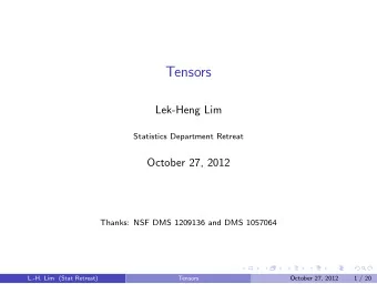
role of tensors in numerical mathematics Lek-Heng Lim University of Chicago February 2, 2015 thanks: NSF DMS 1209136, DMS 1057064, AFOSR FA9550-13-1-0133

what is a tensor? • a tensor is a multilinear functional f : V 1 × · · · × V d → R for k = 1 , . . . , d , f ( v 1 , . . . , α u k + β w k , . . . , v d ) = α f ( v 1 , . . . , u k , . . . , v d ) + β f ( v 1 , . . . , w k , . . . , v d ) • if we give f coordinates, i.e., choose bases on V 1 , . . . , V d , get hypermatrix A = ( a j 1 ··· j d ) ∈ R n 1 ×···× n d where n 1 = dim V 1 , . . . , n d = dim V d • d -dimensional hypermatrix is d -tensor in coordinates • matrix is linear operator/bilinear form/dyad in coordinates

matrix notions may be extended • rank • hyperdeterminant • positive definiteness • rank retaining decompositions • system of multilinear equations • multilinear programming • multilinear least squares • eigenvalues and eigenvectors • singular values and singular vectors • Gaussian elimination and QR factorization • nonnegative tensors and Perron-Frobenius theory • spectral, operator, H¨ older, nuclear norms [L.-H. Lim, “Tensors and hypermatrices,” Chapter 15, 30 pp., in L. Hogben (Ed.), Handbook of Linear Algebra , 2nd Ed., CRC Press, 2013]

matrix operations may be extended • linear combination: A , B ∈ R n 1 ×···× n d , α, β ∈ R , α A + β B = ( α a j 1 ··· j d + β b j 1 ··· j d ) • outer product: A ∈ R n 1 ×···× n d , B ∈ R m 1 ×···× m e , A ⊗ B = ( a i 1 ··· i d b j 1 ··· j e ) ∈ R n 1 ×···× n d × m 1 ×···× m e • contraction: A ∈ R n 1 ×···× n d − 1 × p , B ∈ R p × m 2 ×···× m e , � p � � ∈ R n 1 ×···× n d − 1 × m 2 ×···× m e � A , B � d : 1 = a i 1 ··· i d − 1 k b kj 2 ··· j e k = 1 • all arise from coordinate-free operations on tensors • what about multiplication? e.g. take A , B ∈ R n × n × n and form AB ∈ R n × n × n

tensors are useful

why tensors 1 • d = 0 , 1 , 2: scalars, vectors, matrices • why should you care about d > 2? • comes up more often than you might expect principle of linearity: in almost any natural process, if we make sufficiently small changes, the variation will be linear with respect to the changes principle of multilinearity: in almost any natural process, if we keep all but one factor constant, the principle of linearity will apply to that changing factor 1 succumbing to popular (but erroneous) nomenclature, will use the term ‘tensor’ even when referring to a hypermatrix

derivatives, moments, cumulants • higher-order derivatives ∇ f ( x ) ∈ R n , ∇ 2 f ( x ) ∈ R n × n , f ( x ) ∈ R , ∇ 3 f ( x ) ∈ R n × n × n , ∇ 4 f ( x ) ∈ R n × n × n × n , . . . • higher-order moments E ( x ⊗ x ⊗ · · · ⊗ x ) ∈ R n × n ×···× n • higher-order cumulants m � i | α | κ α ( x ) t α log E ( exp ( i � t , x � )) ≈ α ! | α | = 1 • mean, variance, skewness, kurtosis ( κ α ( x )) | α | = 1 ∈ R n , ( κ α ( x )) | α | = 2 ∈ R n × n , ( κ α ( x )) | α | = 3 ∈ R n × n × n , ( κ α ( x )) | α | = 4 ∈ R n × n × n × n , . . .

principal components of cumulants PCA right singular vectors Principal kurtosis components 0.4 0.4 1 11 0.3 0.2 50 3 14 12 6 24 21 13 3 22 35 33 32 14 10 1 45 25 37 8 16 4 36 7 0.2 0 11 34 39 19 5 45 41 29 27 40 46 47 31 49 18 20 50 26 43 2 44 23 38 15 42 48 30 30 9 19 8 28 38 33 24 0.1 −0.2 43 Comp 2 18 Comp 2 32 28 26 22 21 27 29 40 34 48 31 37 0 41 −0.4 13 17 10 6 44 16 35 47 4 20 15 25 46 −0.1 5 −0.6 49 12 42 23 39 2 −0.2 −0.8 36 17 9 7 −0.3 −1 −0.5 0 0.5 −0.5 0 0.5 1 Comp 1 Comp 1 Figure: all Gaussian except 17 and 39; left: principal components; right: principal kurtosis components (thanks! Rasmus)

quantum mechanics • H 1 , . . . , H d state spaces, state space of unified system is S ⊆ H 1 ⊗ · · · ⊗ H d • S has factorizable states ψ 1 ⊗ · · · ⊗ ψ d and mixed states αψ 1 ⊗ · · · ⊗ ψ d + · · · + βϕ 1 ⊗ · · · ⊗ ϕ d • H j : H j → H j Hamiltonian of j th system and I identity H 1 ⊗ I ⊗ · · · ⊗ I + I ⊗ H 2 ⊗ · · · ⊗ I + · · · + I ⊗ · · · ⊗ I ⊗ H d Hamiltonian of unified system if systems do not interact • indistinguishable systems H 1 = · · · = H d = H : bosons state space of unified system is S d ( H ) ⊆ H ⊗ d fermions state space of unified system is Λ d ( H ) ⊆ H ⊗ d

quarks • V ⊗ V = S 2 ( V ) ⊕ Λ 2 ( V ) • V ⊗ V ⊗ V = S 3 ( V ) ⊕ S ( 2 , 1 ) ( V ) ⊕ S ( 2 , 1 ) ( V ) ⊕ Λ 3 ( V ) • special case: V = C 3 : standard basis of C 3 × 3 × 3 E ijk = e i ⊗ e j ⊗ e k where e 1 , e 2 , e 3 standard basis of C 3 • interpretation e 1 = | u � = state of the u -quark e 2 = | d � = state of the d -quark e 3 = | s � = state of the s -quark E ijk = composite state of the three quark states e i , e j , e k • proton, two u -quarks and one d -quark, has state 2 ( e 1 ⊗ e 1 ⊗ e 2 − e 2 ⊗ e 1 ⊗ e 1 ) ∈ S ( 2 , 1 ) ( C 3 )

latent variables • behind one of the most fundamental graphical models • na¨ ıve Bayes model � Pr ( x , y , z ) = h Pr ( h ) Pr ( x | h ) Pr ( y | h ) Pr ( z | h ) H ◦ • • • X Y Z • e.g. causality inference, phylogenetics

example: phylogenetics • Markov model for 3-taxon tree [Allman–Rhodes, 2003] • probability distribution given by 4 × 4 × 4 table with model P = π A ρ A ⊗ σ A ⊗ θ A + π C ρ C ⊗ σ C ⊗ θ C + π G ρ G ⊗ σ G ⊗ θ G + π T ρ T ⊗ σ T ⊗ θ T • for i , j , k ∈ { A , C , G , T } p ijk = π A ρ Ai σ Aj θ Ak + π C ρ Ci σ Cj θ Ck + π G ρ Gi σ Gj θ Gk + π T ρ Ti σ Tj θ Tk

neuroimaging identify neural fibers as from diffusion MRI data fODF Maxima Schultz–Seidel [T. Schultz, A. Fuster, A. Ghosh, L. Florack, and L.-H. Lim, “Higher-order tensors in diffusion imaging,” pp. 129–161, Visualization and Processing of Tensors and Higher Order Descriptors for Multi-Valued Data , Springer, 2014]

positive decomposition • A = ( a ijkl ) ∈ S 4 ( R n ) , i.e., a ijkl = a ijlk = a jilk = · · · = a lkji • want positive decomposition A = λ 1 v 1 ⊗ v 1 ⊗ v 1 ⊗ v 1 + · · · + λ r v r ⊗ v r ⊗ v r ⊗ v r with r minimal and λ 1 ≥ λ 2 ≥ · · · ≥ λ r > 0 , � v 1 � = · · · = � v r � = 1 • more generally for any even order d ≥ 4 • generalization of symmetric eigenvalue decomposition for positive semidefinite matrices • not always possible — say ‘positively decomposable’ if decomposition exist

diffusion MRI imaging • after preprocessing, MRI signal is f : S 2 → R • f is homogeneous polynomial of even degree, � n f ( x ) = j 1 ,..., j d = 1 a j 1 ··· j d x j 1 · · · x j d ∈ R [ x 1 , . . . , x n ] d • coefficients are hypermatrices A = ( a j 1 ··· j d ) ∈ R n × n ×···× n • model implies f is sum of powers of linear forms � r i = 1 ( v T i x ) d f ( x ) = • equivalently, A positively decomposable � r i = 1 v ⊗ d A = i • v i gives direction of i th fiber in a voxel [L.-H. Lim and T. Schultz, “Moment tensors and high angular resolution diffusion imaging,” preprint , (2015)]

complexity

most tensor problems are NP-hard • some have no FPTAS • some are NP-hard even to approximate • some are #P-hard • some are VNP-complete • some are undecidable • isn’t this bad news? [C. J. Hillar and L.-H. Lim, “Most tensor problems are NP-hard,” Journal of the ACM , 60 (2013), no. 6, Art. 45, 39 pp.]

encoding NP-hard problems 1 2 1 2 4 3 4 3 3-colorings encoded as real solutions to bilinear system: a 1 c 1 − b 1 d 1 − u 2 , b 1 c 1 + a 1 d 1 , c 1 u − a 2 1 + b 2 1 , d 1 u − 2 a 1 b 1 , a 1 u − c 2 1 + d 2 1 , b 1 u − 2 d 1 c 1 , a 2 c 2 − b 2 d 2 − u 2 , b 2 c 2 + a 2 d 2 , c 2 u − a 2 2 + b 2 2 , d 2 u − 2 a 2 b 2 , a 2 u − c 2 2 + d 2 2 , b 2 u − 2 d 2 c 2 , a 3 c 3 − b 3 d 3 − u 2 , b 3 c 3 + a 3 d 3 , c 3 u − a 2 3 + b 2 3 , d 3 u − 2 a 3 b 3 , a 3 u − c 2 3 + d 2 3 , b 3 u − 2 d 3 c 3 , a 4 c 4 − b 4 d 4 − u 2 , b 4 c 4 + a 4 d 4 , c 4 u − a 2 4 + b 2 4 , d 4 u − 2 a 4 b 4 , a 4 u − c 2 4 + d 2 4 , b 4 u − 2 d 4 c 4 , a 2 1 − b 2 1 + a 1 a 3 − b 1 b 3 + a 2 3 − b 2 3 , a 2 1 − b 2 1 + a 1 a 4 − b 1 b 4 + a 2 4 − b 2 4 , a 2 1 − b 2 1 + a 1 a 2 − b 1 b 2 + a 2 2 − b 2 2 , a 2 2 − b 2 2 + a 2 a 3 − b 2 b 3 + a 2 3 − b 2 3 , a 2 3 − b 2 3 + a 3 a 4 − b 3 b 4 + a 2 4 − b 2 4 , 2 a 1 b 1 + a 1 b 2 + a 2 b 1 + 2 a 2 b 2 , 2 a 2 b 2 + a 2 b 3 + a 3 b 2 + 2 a 3 b 3 , 2 a 1 b 1 + a 1 b 3 + a 2 b 1 + 2 a 3 b 3 , 2 a 1 b 1 + a 1 b 4 + a 4 b 1 + 2 a 4 b 4 , 2 a 3 b 3 + a 3 b 4 + a 4 b 3 + 2 a 4 b 4 , w 2 1 + w 2 2 + · · · + w 2 17 + w 2 18 bilinear system: y T A k z = x T B k z = x T C k y = 0, k = 1 , . . . , n

tensors shed light on foundational questions