= Tensors More Examples Entity Keywords Tensor Matrix Relation - PowerPoint PPT Presentation

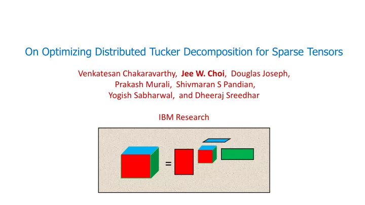
On Optimizing Distributed Tucker Decomposition for Sparse Tensors Venkatesan Chakaravarthy, Jee W. Choi , Douglas Joseph, Prakash Murali, Shivmaran S Pandian, Yogish Sabharwal, and Dheeraj Sreedhar IBM Research =

Tensors More Examples Entity Keywords Tensor Matrix Relation Reviews Entity Users Amazon reviews [LM’13] NELL [CBK+ 13] Image Video Enron Emails [AS ‘04] Sender x Receiver x Word x Date Year Flickr [GSS ‘08] User x Image x Tag x Date Conf Delicious [GSS ‘08] User x Page x Tag x Date Conf Authors Authors

Tucker Decomposition Singular Value Decomposition Σ 𝜏 1 𝜏 2 0 𝑊 𝑈 \sigma 𝑉 ≈ 𝑁 0 𝜏 𝑠 Right singular vectors Singular values Left singular vectors Tucker Decomposition = Higher Order SVD Applications • PCA: Analyze different dimensions • ≈ Text analytics • Computer vision • Signal processing 𝐿 1 × 𝐿 2 × 𝐿 3 𝑀 1 × 𝑀 2 × 𝑀 3

Higher Order Orthonormal Iterator (HOOI) • Initial decomposition – Obtained via HOSVD, STHOSVD, random matrices HOOI 𝐵 − 𝑜𝑓𝑥 𝐶 − 𝑜𝑓𝑥 𝐵 𝐶 + 𝑈 Improve 𝐷 − 𝑜𝑓𝑥 𝐷 • Refinement : improve accuracy • Applied multiple times to get increasing accuracy 4

Prior Work & Objective • Dense tensors [BK’07, ABK’16, CCJ+ 17, JPK’ 15] • Sequential, shared memory and distributed implementations • Sparse tensors [KS’08, BMV+ 12, SK’16, KU’16] • Sequential, shared memory and distributed implementations • [KU’16 ] : First distributed implementation for sparse tensors Our objective • Efficient distributed implementation for sparse tensors • Builds on work of [KU’16] [KS’08] T. Kolda and J. Sun. 2008. Scalable tensor decompositions for multi-aspect data mining. In ICDM. [BMV’12] M. Baskaran, B. Meister, N. Vasilache, and R. Lethin. 2012. Efficient and scalable computations with sparse tensors. In HPEC. [SK’16] S. Smith and G. Karypis. 2017. Accelerating the Tucker Decomposition with Compressed Sparse Tensors. In Euro-Par. [KU’16] O. Kaya and B. Uçar. 2016. High performance parallel algorithms for the Tucker decomposition of sparse tensors. In ICPP.

HOOI – Outline Singular Vectors Matricize 𝑁 1 𝐵 − 𝑜𝑓𝑥 𝐶 𝑈 𝐷 𝑈 X X SVD T 𝐿 1 𝑤𝑓𝑑𝑢𝑝𝑠𝑡 𝑁 2 B −𝑜𝑓𝑥 𝐵 𝑈 𝐷 𝑈 X X SVD T 𝐿 2 𝑤𝑓𝑑𝑢𝑝𝑠𝑡 𝑁 3 C −𝑜𝑓𝑥 𝐵 𝑈 𝐶 𝑈 X X SVD T 𝐿 3 𝑤𝑓𝑑𝑢𝑝𝑠𝑡 T Alternating least squares B A • A Fix B and C. Find Best A. TTM – Tensor times • Fix A and C. Find Best B matrix multiplications • C C B Fix B and C. Find Best C SVD SVD SVD C-new A-new B-new 6

Sparse HOOI : Distribution Schemes and Performance Parameters Sparse HOOI : Distribution Schemes and Performance Parameters Coordinate Coordinate • TTM Component • TTM Component Representation Representation • Computation only • Computation only e1 (1, 2, 1), 0.1 (1, 2, 1), 0.1 • All schemes have same computational load (FLOPs) • All schemes have same computational load (FLOPs) e1 (3, 1, 2), 1.1 (3, 1, 2), 1.1 e5 e5 • Load balance • Load balance e2 (2, 3, 2), 1.2 (2, 3, 2), 1.2 e2 (1, 3, 2), 1.4 (1, 3, 2), 1.4 e6 e6 • SVD Component • SVD Component (1, 1, 2), 3.1 (1, 1, 2), 3.1 e3 e3 (2, 2, 2), 0.5 (2, 2, 2), 0.5 e7 e7 • Both computation and communication • Both computation and communication (3, 2, 1), 0.4 (3, 2, 1), 0.4 e4 e4 e8 e8 (3, 3 1), 0.7 (3, 3 1), 0.7 • Computational load • Computational load • Load balance • Load balance • Communication volume • Communication volume e1 e2 e2 e3 e3 e4 e4 e5 e6 e6 e7 e7 e8 e8 • • e1 e5 Factor Matrix transfer (FM) Factor Matrix transfer (FM) • • Communication only Communication only • • At the end of each HOOI invocation, factor matrix At the end of each HOOI invocation, factor matrix rows need to be communicated among processors rows need to be communicated among processors for the next invocation for the next invocation • • Communication volume Communication volume Proc 1 Proc 1 Proc 2 Proc 2 Proc 3 Proc 3

Prior Schemes • CoarseG - Coarse grained schemes [KU’16] • Allocate entire “slices” to processors • MediumG - Medium grained scheme [SK ‘16] • Grid based partitioning – similar to block partitioning of matrices • FineG - Fine grained scheme [KU’16] • Allocate individual elements using hypergraph partitioning methods TTM SVD FM Dist. time CoarseG Inefficient Efficient Inefficient Fast MediumG Efficient Inefficient Efficient Fast FineG Efficient Inefficient Efficient Slow • Distribution time • CoarseG, MediumG – greedy, fast procedures • FineG – Complex, slow procedure based on sophisticated hypergraph partitioning methods

Our Contributions • We identify certain fundamental metrics • Determine TTM load balance, SVD load and load balance, SVD volume • Design a new distribution scheme denoted Lite Lite • Near-optimal on the fundamental metrics • Near-optimal on • Only parameter not optimized is FM volume • TTM load balance • Computation time dominates • SVD load and load balance • So, Lite performance better • SVD communication volume • Lightweight procedure with fast distribution time • Performance gain up to 3x TTM SVD FM Dist. time CoarseG Inefficient Efficient Inefficient Fast MediumG Efficient Inefficient Efficient Fast FineG Efficient Inefficient Efficient Slow Lite Near- Near- Inefficient Fast optimal Optimal

Mode 1 – Sequential TTM T B A A Penultimate TTM matrix C C B 𝐶 𝑈 𝐷 𝑈 𝑁 X X T SVD A-new SVD SVD SVD C-new A-new B-new Kronecker product (1, -, -) e1 ෢ 𝐿 1 Involves factor matrices (2, -, -) e2 • Slice – elements with same 1 (1, -, -) e3 coordinate; same color L 1 (3, -, -) • e4 Each slice updates the 2 corresponding row in the (3, -, -) e5 3 penultimate matrix (1, -, -) e6 (2, -, -) e7 Penultimate Matrix M (3, -, -) e8

Distributed TTM Penultimate matrix is sum-distributed Local copy 1 (1, -, -) e1 Proc 1 (2, -, -) e2 2 (1, -, -) e3 3 Local copy 1 1 (3, -, -) e4 2 Proc 2 (3, -, -) e5 2 (1, -, -) 3 e6 3 Penultimate Matrix M Local copy 1 (2, -, -) e7 Proc 3 (3, -, -) e8 2 3

SVD via Lanczos Method • Lanczos method provides a vector x in . Return x out = Z x in . 0 𝑦 𝑝𝑣𝑢 • Done implicitly over the sum-distributed matrix Local copy 1 (1, -, -) 1 e1 2 = x 𝑦 𝑗𝑜 (2, -, -) 2 Proc 1 e2 3 (1, -, -) 3 e3 1 𝑦 𝑝𝑣𝑢 𝑦 𝑝𝑣𝑢 Local copy 1 (3, -, -) 1 e4 1 P 1 2 x 𝑦 𝑗𝑜 Proc 2 = 2 (3, -, -) e5 2 P 3 3 3 (1, -, -) e6 3 P 2 2 𝑦 𝑝𝑣𝑢 Owners Local copy 1 1 (2, -, -) e7 2 Proc 3 = x 𝑦 𝑗𝑜 2 (3, -, -) e8 3 3 TTM Computation SVD Computation

Performance Metrics Along Each Mode TTM 1 𝑎 1 Local copy • TTM-LImb 1 • Max number of elements assigned to the (1, -, -) e1 processors Proc 1 (2, -, -) e2 2 • Optimal value – E / P (1, -, -) e3 3 • Number of elements / Number of processors 2 SVD 𝑎 1 Local copy • SVD-Redundancy 1 (3, -, -) e4 • Total number of times slices are shared Proc 2 (3, -, -) e5 2 • Measures computational load, comm volume (1, -, -) e6 • Optimal value = L (length along the mode) 3 • SVD-LImb: • Max number of slices shared by the processors 3 𝑎 1 Local copy • Optimal value = L / P 1 (2, -, -) e7 Factor Matrix Transfer Proc 3 (3, -, -) e8 • Communication volume at the each iteration 2 3 TTM-Limb = 3 (optimal) SVD-Red = 6 (optimal = 3) SVD-Limb = 2 (optimal =1)

Prior Schemes • Uni-policy Schemes • A single policy for computation along all modes • Only a single copy of the tensor need to be stored • Less memory footprint, but less optimization opportunities • Multi-policy Schemes • Independent distribution for each mode • N copies need to be stored, one along each mode • More memory footprint, but more optimization opportunities • Coarse-grained Scheme [Kaya- Ucar’16] • Allocate each slice in entirety to a processor. No slice-sharing • Medium-grained Scheme [Smith et al ‘16] • Grid partitioning proposed in CP context • Hyper-graph Scheme (Fine-grained) [Kaya-Ucar ‘16] • All issues captured via a hyper-graph • Find min-cut partitioning

Our Scheme - Lite

Lite - Results • Near-optimal • TTM-Limb • TTM-Limb = E / P (optimal) • SVD computational load, load balance • SVD-Redundancy = L + P (optimal = L) • SVD communication volume • SVD-Limb = L/P + 2 (optimal = L/P) • Only issue is high factor matrix transfer volume • Computation dominates. So, not an issue. CoarseG MediumG FineG Lite Type Multi-policy Uni-policy Uni-policy Multi-policy Distribution time Greedy Greedy Complex (Slow) Greedy (fast) (fast) (fast) TTM-Limb High Reasonable Reasonable Optimal SVD- Optimal High Reasonable Optimal Redundancy SVD-Limb Reasonable Reasonable High Optimal SVD-Volume Optimal Reasonable Reasonable Optimal FM-Volume High Reasonable Reasonable High

Experimental Evaluation • R92 cluster – 2 to 32 nodes. • 16 MPI ranks per node, each mapped to a core. So, 32 to 512 MPI ranks • Dataset : FROSTT repository