Robustness measures and level set methods P. Van Dooren Abstract In - PDF document

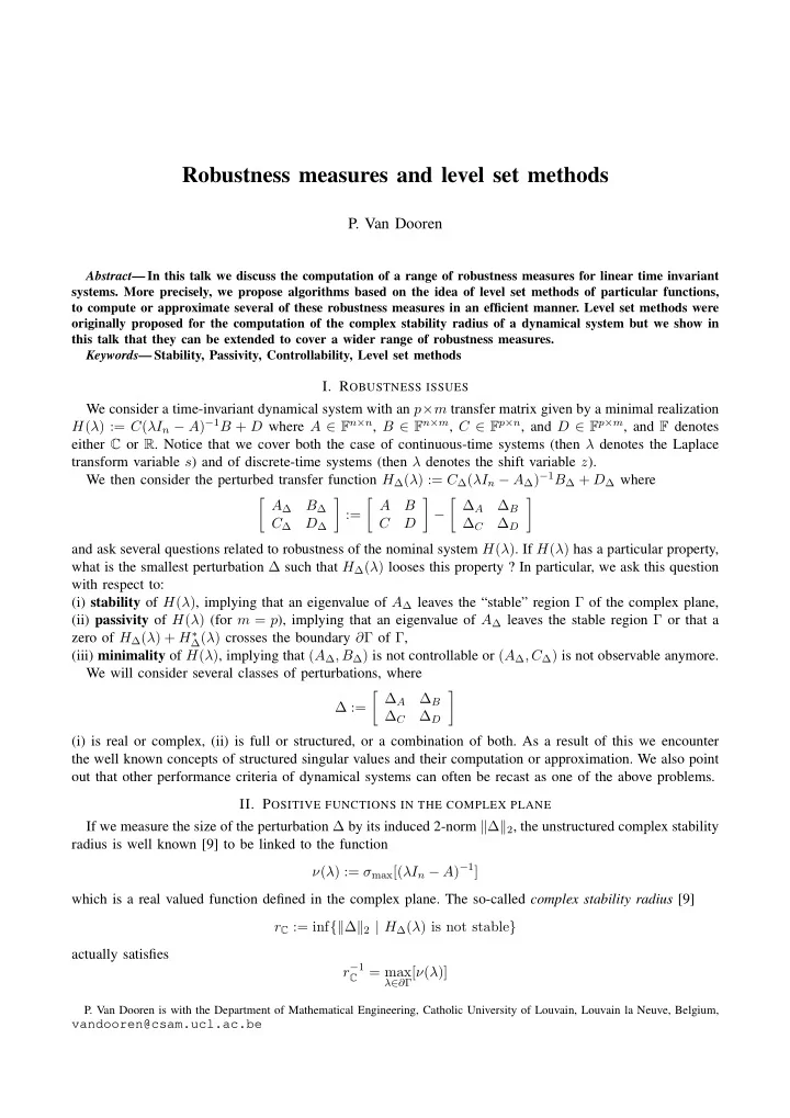
Robustness measures and level set methods P. Van Dooren Abstract — In this talk we discuss the computation of a range of robustness measures for linear time invariant systems. More precisely, we propose algorithms based on the idea of level set methods of particular functions, to compute or approximate several of these robustness measures in an efficient manner. Level set methods were originally proposed for the computation of the complex stability radius of a dynamical system but we show in this talk that they can be extended to cover a wider range of robustness measures. Keywords — Stability, Passivity, Controllability, Level set methods I. R OBUSTNESS ISSUES We consider a time-invariant dynamical system with an p × m transfer matrix given by a minimal realization H ( λ ) := C ( λI n − A ) − 1 B + D where A ∈ F n × n , B ∈ F n × m , C ∈ F p × n , and D ∈ F p × m , and F denotes either C or R . Notice that we cover both the case of continuous-time systems (then λ denotes the Laplace transform variable s ) and of discrete-time systems (then λ denotes the shift variable z ). We then consider the perturbed transfer function H ∆ ( λ ) := C ∆ ( λI n − A ∆ ) − 1 B ∆ + D ∆ where � A ∆ � A � ∆ A � � � ∆ B B ∆ B := − C ∆ D ∆ C D ∆ C ∆ D and ask several questions related to robustness of the nominal system H ( λ ) . If H ( λ ) has a particular property, what is the smallest perturbation ∆ such that H ∆ ( λ ) looses this property ? In particular, we ask this question with respect to: (i) stability of H ( λ ) , implying that an eigenvalue of A ∆ leaves the “stable” region Γ of the complex plane, (ii) passivity of H ( λ ) (for m = p ), implying that an eigenvalue of A ∆ leaves the stable region Γ or that a zero of H ∆ ( λ ) + H ∗ ∆ ( λ ) crosses the boundary ∂ Γ of Γ , (iii) minimality of H ( λ ) , implying that ( A ∆ , B ∆ ) is not controllable or ( A ∆ , C ∆ ) is not observable anymore. We will consider several classes of perturbations, where � ∆ A � ∆ B ∆ := ∆ C ∆ D (i) is real or complex, (ii) is full or structured, or a combination of both. As a result of this we encounter the well known concepts of structured singular values and their computation or approximation. We also point out that other performance criteria of dynamical systems can often be recast as one of the above problems. II. P OSITIVE FUNCTIONS IN THE COMPLEX PLANE If we measure the size of the perturbation ∆ by its induced 2-norm � ∆ � 2 , the unstructured complex stability radius is well known [9] to be linked to the function ν ( λ ) := σ max [( λI n − A ) − 1 ] which is a real valued function defined in the complex plane. The so-called complex stability radius [9] r C := inf {� ∆ � 2 | H ∆ ( λ ) is not stable } actually satisfies r − 1 = max λ ∈ ∂ Γ [ ν ( λ )] C P. Van Dooren is with the Department of Mathematical Engineering, Catholic University of Louvain, Louvain la Neuve, Belgium, vandooren@csam.ucl.ac.be

In Figure 1a we show the function ν ( λ ) for λ ∈ C corresponding to a discrete-time system of order n = 20 . The inverse of the stability radius is the maximum of that function on the unit circle (i.e. on ∂ Γ ). Figure 1b shows the contour plot of the same function and also displays the unit circle, on which this function has to be maximized. This contour plot is also known to correspond to the spectral value sets (or pseudo-spectrum) of the matrix A [18]. 2 1.5 1 0.5 0 −0.5 −1 −1.5 −2 −2 −1 0 1 2 Fig. 1. ν ( λ ) for a stable discrete time system, and the corresponding contour plot If we parameterize ∂ Γ as a function of a real variable ω ( e jω for a discrete-time system and jω for a continuous-time system), then we are actually computing the maximum of a real valued functions of a real variable ω . This is depicted in Figure 2. Frequency response amplitude |H(e j ω )| 40 35 30 25 20 15 10 5 0 −4 −3 −2 −1 0 1 2 3 4 ν ( e jω ) as a function of ω Fig. 2.

III. B ASIC LEVEL SET METHOD The basic idea of level set methods is quite simple. Rather than trying to find the maximum of the above real valued function, one “cuts” with a level ξ and computes the points of intersection. These turn out to be the roots of a particular eigenvalue problem associated with the dynamical system H ( λ ) [5]. 0.8 0.7 0.6 ξ 0 ≡ ξ old 0.5 0.4 0.3 0.2 ω 2 ω 3 ω 1 ω 4 ω 5 ω 6 ω 7 ω 8 0.1 0 1 2 10 10 10 Frequency Singular values σ 1 ( ω ) and σ 2 ( ω ) Fig. 3. In Figure 3, we show the two largest singular value functions σ i ( ω ) for a matrix coming from a continuous- time system. We also indicate a level ξ 0 for which we want to check if there is any eigenvalue σ i ( ω ) = ξ 0 . One easily shows that the supremum ξ max of all levels for which there are still intersections, actually equals r − 1 C . Using this idea, a bisection-based algorithm to find ξ max was derived in [5]. This algorithm has linear convergence. A method with more rapid convergence can be obtained by using additional information on the above singular functions (see [3], [4], [7], [15]). which are obtained as a by-product of the eigenvalue problem used to compute the intersection ω i . In [6] it is shown how to use the information of the derivative of σ max ( ω ) at each point in order to determine the relevant “level sets” [ ω 1 , ω 4 ] and [ ω 5 , ω 8 ] in which one needs to find the maximum of the function σ max ( ω ) . Using these level sets and the derivative of σ max ( ω ) at their endpoints, one then constructs a new frequency ω new that is a good estimate of an extremal frequency of the largest of all singular values. It is shown in [6] that such a scheme has global linear convergence and at least cubic asymptotic convergence. The complexity of each iteration is only cubic in the dimensions of the system matrix of H ( λ ) and reliable numerical methods are now available to solve the underlying eigenvalue problems [1]. IV. E XTENSIONS TO OTHER PROBLEMS The above basic level set method works for problems in which the plotted functions are singular values σ i ( H ( λ )) plotted against λ = jω of e jω , and where H ( λ ) is a rational matrix function. In most of the other

problems we mentioned above, this does not hold anymore. The real stability radius problem and the passivity radius problem both involve a function µ ( H ( λ )) plotted against λ = jω of e jω which at each frequency ω is itself the result of an optimization problem over some other scaling parameters which are elements of a matrix D . For the real stability radius, this is e.g. [14] �� �� ℜ M − d ℑ M µ ( M ) = inf d ∈ (0 , 1] σ 2 d − 1 ℑ M ℜ M involving only a single scalar parameter d . It is also known that µ ( ω ) is then not necessarily continuous anymore (see [6]) and that the problem is much more delicate. Nevertheless, it was shown in [17] that one can still use level set methods to solve this problem. It turns out that the function µ ( ω ) – depicted in Figure 4 as λ γ ( H ( ω )) – is the lower envelope of a set of other functions µ d ( ω ) – depicted in Figure 4 as λ max ( H γ o ( ω )) – which do correspond to a rational matrix function H γ o ( λ )) . The corresponding dotted curves are then smooth even though the lower envelope can be discontinuous [14]. One shows [17] that this can be exploited efficiently to again come up with en efficient level set method for computing the real stability radius. The basic idea is to find the level set of the dotted curve, which is tangential in at least one point with the full curve (which is the lower envelope of all dotted curves). In Figure 4 this yields two possible intervals in which to look for the supremum of the full curve. By doing this, one needs to solve the optimization problem in the scaling parameters D in only a limited number of frequencies and one shows that overall the complexity is still quite low. 2.2 λ max (H γ ( ω )) 2 o 1.8 1.6 1.4 1.2 ξ λ γ (H( ω )) 1 0.8 0.6 0.4 0.2 0 1 2 3 4 5 6 7 8 ω Fig. 4. Level set iterations In the computation of the passivity radius, a very similar problem occurs, except that for the complex passivity radius problem a single real parameter enters the picture, while for the real passivity radius two real parameters are involved [11], [16]. One can also link this problem tho that of finding a particular performance radius of a closed loop system [10].