Level set methods for robustness measures P. V AN D OOREN CESAME, - PowerPoint PPT Presentation
Level set methods for robustness measures P. V AN D OOREN CESAME, Universit e catholique de Louvain joint work with Y. Genin, T. Lawrence, M. Overton, J. Sreedhar, A. Tits What it is about Fast and reliable computation of robustness measures
Level set methods for robustness measures P. V AN D OOREN CESAME, Universit´ e catholique de Louvain joint work with Y. Genin, T. Lawrence, M. Overton, J. Sreedhar, A. Tits
What it is about Fast and reliable computation of robustness measures for • Stability • Passivity • Minimality for (possibly structured) perturbations { ∆ A , ∆ B , ∆ C , ∆ D } of a (real or complex) plant { A, B, C, D }
Link to structured singular values In each of these problems we need to find a point λ ∈ C such that some singular value or eigenvalue of matrices derived from � � � � A − λI A − λI B A − λI A − λI B C C D is minimal. Level sets (parameterized by ξ ) are sets where singular values or eigenvalues are larger than the parameter ξ . This is clearly related to so-called pseudo-spectra
Setting Given a minimal system G ( λ ) := C ( λI − A ) − 1 B + D and a perturbed system G ∆ ( λ ) := C ∆ ( λI − A ∆ ) − 1 B ∆ + D ∆ we measure perturbations using ∆ A ∆ B A ∆ B ∆ A B := − ∆ := ∆ C ∆ D C ∆ D ∆ C D and use the � ∆ � 2 norm All matrices can be real or complex
Complex stability radius We are looking for the radius r C = inf ∆ {� ∆ � 2 | A ∆ is unstable } (Hinrichsen-Pritchard) We need to find an eigenvalue λ of A ∆ in the unstable region Γ or on its boundary ∂ Γ : det( A + ∆ A − λI ) = 0 , λ ∈ ∂ Γ For the complex case, perturbation theory says � ∆ A � 2 = σ min ( A − λI ) so we have (cfr pseudospectrum) r C = min λ ∈ ∂ Γ σ min ( A − λI ) = 0 , λ ∈ ∂ Γ
Resolvant In systems theory we are more familiar with the resolvent and its norm : G ( λ ) := ( λI − A ) − 1 , r − 1 = max λ ∈ ∂ Γ σ max [ G ( λ )] C 2 1.5 1 0.5 0 −0.5 −1 −1.5 −2 −2 −1 0 1 2
Complex stability radius We wanted the radius r C ( A ) = inf ∆ ∈ C m × p {� ∆ � 2 | A + ∆ A is unstable } We needed to find an eigenvalue λ of A + ∆ A in the unstable region Γ or on its boundary ∂ Γ : det( A + ∆ A − λI ) = 0 , λ ∈ ∂ Γ For the complex case, this depended on the transfer function G ( λ ) = ( λI − A ) − 1 and yielded r − 1 = max λ ∈ ∂ Γ σ max [ G ( λ )] C
Structured stability radius If we impose a very simple structure, the problem becomes r C ( A, B, C ) := ∆ ∈ C m × p {� ∆ � 2 : A + B ∆ C is stable } inf Define G ( λ ) := C ( λI − A ) − 1 B then r − 1 C ( A, B, C ) = max λ ∈ ∂ Γ { σ max [ G ( λ )] } See Hinrichsen Pritchard for more on this
Maximum frequency response We thus need a reliable algorithm to find ( λ ∈ ∂ Γ = jω or e jω ): σ max C ( e jω I − A ) − 1 B max ω Amplitude of frequency response H(e j ω ) 16 Alternative : gradient search 14 but too many peaks may cost 12 a lot and may be trouble- 10 some 8 The solution is to look at the 6 ξ level set 4 −4 −3 −2 −1 0 1 2 3 4
Maximum frequency response We thus need a reliable algorithm to find ( λ ∈ ∂ Γ = jω or e jω ): σ max C ( e jω I − A ) − 1 B max ω Amplitude of frequency response H(e j ω ) 16 Alternative : gradient search 14 but too many peaks may cost 12 a lot and may be trouble- ξ 10 some 8 The solution is to look at the 6 ξ level set 4 −4 −3 −2 −1 0 1 2 3 4
Bisection 0.8 The intersection points ω i with the ξ level (of all singular values) are 0.7 imaginary eigenvalues of a Hamil- 0.6 tonian (or symplectic) matrix ξ 0 ≡ ξ old 0.5 − BB ∗ /ξ A 0.4 H ( ξ ) := C ∗ C/ξ − A ∗ 0.3 This can be used to do e.g. bisection 0.2 Linear convergence (Byers) ω 2 ω 3 ω 1 ω 4 ω 5 ω 6 ω 7 ω 8 0.1 0 1 2 10 10 10 Frequency Interval midpoint rule is quadratic (Boyd et al, Bruinsma et al)
Correct intervals and interpolation Two dominant singular values 12 10 The eigenvalue problem also yields 8 the derivatives of the singular value 6 plots 4 They yield the info to find each indi- 2 vidual singular value 0 −4 −3 −2 −1 0 1 2 3 4 frequency
Correct intervals and interpolation Two dominant singular values 12 10 The eigenvalue problem also yields 8 the derivatives of the singular value 6 plots 4 They yield the info to find each indi- 2 vidual singular value 0 −4 −3 −2 −1 0 1 2 3 4 frequency
Midpoint vs interpolation Acceleration techniques yielding superlinear convergence midpoint rule fmid=12.76, fint=12.82 Midpoint rule (Boyd et al) 13 Choose ω + as midpoint of interval 12.5 Choose ξ + as function at that ω + 12 | ξ + − ξ ∗ | = O | ξ − ξ ∗ | 2 11.5 σ max 11 Interpolation rule (Genin-V) 10.5 Choose ξ ++ as maximum of 10 cubic interpolating polynomial 2 2.2 2.4 2.6 2.8 3 | ξ ++ − ξ ∗ | = O | ξ − ξ ∗ | 4 frequency
Quartic convergence Iteration ξ (midp.) Intervals (midp.) ξ (cubic) Intervals (cubic) 1 0.5224 [0,1.1991] 0.5224 [0,1.1991] 2 0.7980 [0.1867,0.5995] [0.7097,1.0153] 6.5148 [0.7804,0.7994] 3 1.7669 [0.7472,0.8625] 8.4043 [0.78942,0.78943] 4 5.3027 [0.7762,0.8048] 8.4043 Convergence 5 8.3691 [0.7884,0.7905] 6 8.4043 [0.78942,0.78943] Complexity results (per iteration): a (2 n ) 3 , ω i : a ≈ 50 (exploit Hamiltonian structure) bn 2 , ∂σ j /∂ω : b < n (exploit Hamiltonian structure) cn 2 ( m + p ) , ξ k : c < n (use condensed forms) Overall complexity is O ( n ) 3
Real stability radius r R ( A, B, C ) := ∆ ∈ R m × p {� ∆ � 2 : A + B ∆ C is stable } inf Define G ( λ ) := C ( λI − A ) − 1 B and G := G r + iG i then (Qiu et al) r − 1 R ( A, B, C ) = sup λ ∈ ∂ Γ { µ R [ G ( λ )] } where G r − γG i µ R ( G ) := γ ∈ (0 , 1] σ 2 [ P γ ] := inf γ ∈ (0 , 1] σ 2 inf G i /γ G r
Associated Hamiltonian We use I γI G r − γG i G 0 , = T γ T γ 1 T γ := √ 2 I/γ − I G i /γ G r 0 G to derive an associated real Hamiltonian matrix αBB T − βBB T A 0 − βBB T αBB T 0 − A H γ ( ξ ) := − αC T C βC T C − A T 0 βC T C − αC T C A T 0 where α := (1 + γ 2 ) / (2 γξ ) , β := (1 − γ 2 ) / (2 γξ ) We can find the jω eigenvalue of H γ ( ξ ) that correspond to σ 2 [ P γ ( ω )]
Lower envelope For each γ o value there is a σ 2 plot whose levels we can check with H γ o ( ξ o ) The (solid) curve µ R ( ω ) we need 2.2 λ max (H γ ( ω )) to maximize is the lower envelope 2 o of these (dotted) curves 1.8 1.6 1.4 Each one is tangent to µ R ( ω ) in 1.2 ξ λ γ (H( ω )) one frequency ω o 1 0.8 Convergence is quadratic or cubic 0.6 0.4 (Sreedhar-Tits-V) 0.2 0 1 2 3 4 5 6 7 8 ω
Passivity radius Let G ( λ ) := C ( λI n − A ) − 1 B + D be strictly passive i.e. stable and positive real G ( jω ) + [ G ( jω )] ∗ ≻ 0 , ∀ ω ∈ R Re λ i ( A ) < 0 , Consider the perturbed system G ∆ ( λ ) := C ∆ ( λI n − A ∆ ) − 1 B ∆ + D ∆ We wish to find the passivity radius of the system G ( λ ) pr C ( G ) := inf ∆ {� ∆ � 2 | G ∆ ( λ ) is not passive } .
KYP lemma Passivity (stability and positive realness) G ∆ ( jω ) + [ G ∆ ( jω )] ∗ ≻ 0 , Re λ i ( A ) < 0 , ∀ ω ∈ R iff there exists a Hermitian matrix P such that − A ∆ P − PA ∗ B ∆ − PC ∗ ∆ ∆ ≻ 0 , P ≻ 0 B ∗ ∆ − C ∆ P D ∆ + D ∗ ∆ Stability Re λ i ( A ) < 0 iff there exists a Hermitian matrix P such that − A ∆ P − PA ∗ ∆ ≻ 0 , P ≻ 0 Therefore stability can not be lost “before” positive realness is lost (It can at one frequency if minimality is also lost)
Positive realness G ∆ ( jω ) + [ G ∆ ( jω )] ∗ ≻ 0 gets lost as soon as 0 A ∆ − jωI n B ∆ det = 0 , for some ω ∈ R A ∗ C ∗ ∆ + jωI n 0 ∆ B ∗ C ∆ D ∆ + D ∗ ∆ ∆ or as soon as 0 ∆ E T = 0 det H ω + E ∆ ∗ 0 where 0 A − jωI n B I n 0 0 0 A ∗ + jωI n H ω := , E := C ∗ 0 0 0 I n 0 B ∗ D + D ∗ C 0 I m 0 I m
We need a closed expression for 0 ∆ E T = 0 min � ∆ � 2 : det H ω + E ∆ ∗ 0 The corresponding transfer function is H ( ω ) := E T H ( ω ) − 1 E and one shows (Hu-Qiu, Overton-V) that the passivity radius is then pr − 1 C ( A, B, C, D ) = sup ω { ν C [ H ( ω )] } where ν C := max { inf γ λ max ( H γ ) , inf γ λ max ( − H γ ) } and γI n + m 0 H γ := T γ HT γ , T γ := 0 I n + m /γ
Associated Hamiltonian For each γ o value there is a λ max plot whose levels we can check with − γ 2 ( D + D ∗ − γ 2 o + γ − 2 o I n /ξ o A − jωI n B I ) − 1 � � B ∗ C o − A ∗ + jωI n ξ o − γ − 2 o I n /ξ o C ∗ 2.2 λ max (H γ ( ω )) 2 o The (solid) curve is the lower enve- 1.8 lope of the dotted curves and each 1.6 one is tangent to it in one frequency 1.4 1.2 ξ λ γ (H( ω )) ω o 1 0.8 Convergence is quadratic or cubic 0.6 (Overton-V) 0.4 0.2 0 1 2 3 4 5 6 7 8 ω
Recommend
More recommend
Explore More Topics
Stay informed with curated content and fresh updates.
