Robust estimation techniques in computer vision Vasile Gui July - PowerPoint PPT Presentation
Robust estimation techniques in computer vision Vasile Gui July 2019 UPT University 'Politehnica' Timisoara Goals of CV: evaluating and recognizing image content Prior to obtaining semantics from images, we need to extract: locations;
Robust estimation techniques in computer vision Vasile Gui July 2019 UPT University 'Politehnica' Timisoara
Goals of CV: evaluating and recognizing image content Prior to obtaining semantics from images, we need to extract: • locations; • shapes of geometric objects in an image; • motions in a video sequence; • or projective transformations between images of the same scene; • Etc.
What have in common all these applications? • Presence of noise • Neighbourhood processing involved
What have in common all these applications? • Presence of noise • Neighbourhood processing involved • The neighbourhood may contain more objects • Without prior segmentation it is unclear what we measure in the window.
What have in common all these applications? • Presence of noise • Neighbourhood processing involved • The neighbourhood may contain more objects • Without prior segmentation it is unclear what we measure in the window. • RE can alleviate this chicken and egg problem.
Some CV applications using RE
Reconstruction: 3D from photo collections Q. Shan, R. Adams, B. Curless, Y. Furukawa, and S. Seitz, The Visual Turing Test for Scene Reconstruction, 3DV 2013 YouTube Video From Svetlana Lazebnik
Reconstruction: 4D from photo collections R. Martin-Brualla, D. Gallup, and S. Seitz, Time-Lapse Mining from Internet Photos, SIGGRAPH 2015 YouTube Video From Svetlana Lazebnik
Outline • Introducing RE from an image filtering perspective • M estimators • Maximum likelihood estimators (MLE) • Kernel density estimators (KDE) • The RANSAC family • Some examples and conclusions • Not a survey of RE in CV • Raising awareness about RE
Robust estimation A detail preserving image smoothing perspective
Image smoothing filter goal: Generate a smoothed image from a noisy image
Image smoothing filter goal: Generate a smoothed image from a noisy image Usual assumptions: – Noise is changing randomly - unorganized – Useful image part: piecewise smooth
Smoothing filter approach: For each pixel: – Define a neighbourhood (window) – Estimate central pixel ’ s “ true ” value using all pixels in the window – Assumption: the estimate should be “ similar ” to pixels in the window – Filters differ in similarity definition
What is the problem? • The processing window may contain more objects or distinctive parts of an object.
What is the problem? • The processing window may contain more objects or distinctive parts of an object. • This violates the assumption of similarity with central pixel.
What is the problem? • The processing window may contain more objects or distinctive parts of an object. • This violates the assumption of similarity with central pixel. • If we average pixels, we reduce the effect of random noise …
What is the problem? • The processing window may contain more objects or distinctive parts of an object. • This violates the assumption of similarity with central pixel. • If we average pixels, we reduce the effect of random noise … • but we blur the image and lose some meaningful details.
Some filter comparisons Original noisy mean 5x5 binomial 5x5 median 5x5
Why did the median filter a better job? • Preserving edges • Cleaning “ salt and pepper ” noise
Why did the median filter a better job? • Preserving edges • Robust estimation perspective of the • Cleaning “ salt and question pepper ” noise
M estimator for filter design Huber, P. J. (2009). Robust Statistics. John Wiley & Sons Inc. Pixels: color vectors in a window: 𝐠 𝑗 Estimated color: መ 𝐠 𝑗 = 𝐠 𝑗 − መ Residuals: 𝑠 𝐠 Loss function: 𝜍 𝑣 Minimize loss: መ 𝐠 = argminσ 𝑗𝜗𝑋 𝜍(𝑠 𝑗 )
M estimator for filter design Huber, P. J. (2009). Robust Statistics. John Wiley & Sons Inc. Pixels: color vectors in a window: 𝐠 𝑗 Estimated color: መ 𝐠 𝑗 = 𝐠 𝑗 − መ Residuals: 𝑠 𝐠 Loss function: 𝜍 𝑣 Minimize loss: መ 𝐠 = argminσ 𝑗𝜗𝑋 𝜍(𝑠 𝑗 ) Least squares (LS) loss: 𝜍 𝑣 = 𝑣 2
M estimator for filter design Huber, P. J. (2009). Robust Statistics. John Wiley & Sons Inc. Pixels: color vectors in a window: 𝐠 𝑗 Estimated color: መ 𝐠 𝑗 = 𝐠 𝑗 − መ Residuals: 𝑠 𝐠 Loss function: 𝜍 𝑣 Minimize loss: መ 𝐠 = argminσ 𝑗𝜗𝑋 𝜍(𝑠 𝑗 ) Least squares (LS) loss: 𝜍 𝑣 = 𝑣 2 Solution: መ 𝐠 = σ 𝑗𝜗𝑋 𝐠 𝑗 / σ 𝑗𝜗𝑋 1 i.e. the mean
M estimator for filter design Weighted LS : 𝜍 𝑣 𝑗 = 𝑥 𝑗 (𝑣 𝑗 ) 2 Solution: መ 𝐠 = σ 𝑗𝜗𝑋 𝑥 𝑗 𝐠 𝑗 /σ 𝑗𝜗𝑋 w 𝑗 i.e. the weighted mean
M estimator for filter design Weighted LS : 𝜍 𝑣 𝑗 = 𝑥 𝑗 (𝑣 𝑗 ) 2 Solution: መ 𝐠 = σ 𝑗𝜗𝑋 𝑥 𝑗 𝐠 𝑗 /σ 𝑗𝜗𝑋 w 𝑗 i.e. the weighted mean • Can be any convolution filter, including binomial, if weights depend on distance to window center.
M estimator for filter design Weighted LS : 𝜍 𝑣 𝑗 = 𝑥 𝑗 (𝑣 𝑗 ) 2 Solution: መ 𝐠 = σ 𝑗𝜗𝑋 𝑥 𝑗 𝐠 𝑗 /σ 𝑗𝜗𝑋 w 𝑗 i.e. the weighted mean • Can be any convolution filter, including binomial, if weights depend on distance to window center. • Weights for the bilateral filter depend on distance in space-value domain from central pixel.
M estimator for filter design Absolute value loss: 𝜍 𝑣 = 𝑣 Suppose gray value images, so the loss function has derivative – sign( u ).
M estimator for filter design Absolute value loss: 𝜍 𝑣 = 𝑣 Suppose gray value images, so the loss function has derivative – sign( u ). Solution: σ 𝑗𝜗𝑋 I( መ f > f 𝑗 ) = σ 𝑗𝜗𝑋 I( መ f < f 𝑗 ) , Equal number of lower and higher values than the estimate, i.e. the median : middle of the ordered set.
Why did the median filter outperform convolution filters?
Why did the median filter outperform convolution filters? Outlier samples in the filtering window have less influence on the median than on the weighted mean.
Why did the median filter outperform convolution filters? Outlier samples in the filtering window have less influence on the median than on the weighted mean. Influence function (IF) of a linear filter: = 2 ( ) u w u ( ) d u = ( ) u = ( ) 2 u w u du
Why did the median filter outperform convolution filters? Outlier samples in the filtering window have less influence on the median than on the weighted mean. Influence function (IF) of a linear filter: = 2 ( ) u w u ( ) d u = ( ) u = ( ) 2 u w u du Any sample can have unbounded effect on the estimate (not robust!)
Why did the median filter outperform convolution filters? Outlier samples in the filtering window have less influence on the median than on the weighted mean. Influence function (IF) of a linear filter: = 2 ( ) u w u ( ) d u = ( ) u = ( ) 2 u w u du Any sample can have unbounded effect on the estimate (not robust!) Higher residual sample - higher influence (!!!)
Loss function and IF of the median filter = ( ) | | u u 1, 0 u = = = ( ) ( ) 0, 0 u sign u u − 1, 0 u Bounded (and equal) influence of all samples.
Loss function and IF of the median filter = ( ) | | u u 1, 0 u = = = ( ) ( ) 0, 0 u sign u u − 1, 0 u Bounded (and equal) influence of all samples. Brake down point (BP): number of points arbitrarily deviated causing arbitrarily big estimation error. Median BP: 50%.
Loss function and IF of the median filter = ( ) | | u u 1, 0 u = = = ( ) ( ) 0, 0 u sign u u − 1, 0 u Bounded (and equal) influence of all samples. Brake down point (BP): number of points arbitrarily deviated causing arbitrarily big estimation error. Median BP: 50%. Linear filters: 0%: one very bad outlier is enough … Note, the vector median is a different story.
Should we always use the sample median?
Should we always use the sample median? • When data do not contain outliers the mean has better performance.
Should we always use the sample median? • When data do not contain outliers the mean has better performance. • We want estimators combining the low variance of the mean at normal distributions with the robustness of the median under contamination.
Should we always use the sample median? • When data do not contain outliers the mean has better performance. • We want estimators combining the low variance of the mean at normal distributions with the robustness of the median under contamination. • Let us compare the two filters also from the maximum likelihood perspective!
How can we design robust loss functions?
How can we design robust loss functions? • We need a way to cope with the presence of outlier data, while keeping the efficiency of a classical estimator for normal data.
Recommend
More recommend
Explore More Topics
Stay informed with curated content and fresh updates.
