Robot Motion Planning George Konidaris gdk@cs.brown.edu Fall 2019 - PowerPoint PPT Presentation
Robot Motion Planning George Konidaris gdk@cs.brown.edu Fall 2019 The Planning Problem Finding a sequence of actions to achieve some goal. Classical Planning (define (problem pb3) (:domain blocksworld) (:objects a b c) (:init (on-table a)
Robot Motion Planning George Konidaris gdk@cs.brown.edu Fall 2019
The Planning Problem Finding a sequence of actions to achieve some goal.
Classical Planning (define (problem pb3) (:domain blocksworld) (:objects a b c) (:init (on-table a) (on-table b) (on-table c) (clear a) (clear b) (clear c) (arm-empty)) (:goal (and (on a b) (on b c)))) A B B A C C
Robot Motion Planning
Motion Planning
Motion Planning
Motion Planning
Motion Planning ?? start pose goal
Configuration Space Robot has a configuration space (C-space) : • Values for each joint • Overall pose of reference frame
Configuration Spaces Each joint is a dimension of the configuration space. Let’s say we have a robot with a movable base, and an arm with two revolute joints.
Configuration Spaces Each joint is a dimension of the configuration space. Let’s say we have a robot with an arm with two revolute joints. Configuration space: • x, y, theta of base frame • angle of first joint • angle of second joint A configuration is a setting of values to these 5 variables. Configuration space is the space of all such settings .
Configuration Space Obstacles are no-go regions of configuration space. (images from Wikipedia)
Configuration Space Obstacles are no-go regions of configuration space. (images from Wikipedia)
Configuration Space [via JC LaTombe]
Problem Definition Given : • Configuration space • Start point in C-space • Goal region in C-space • Set of obstacles • Dense regions of 3D-space • ( Also regions of C-space) Find : feasible , obstacle-free (possibly cost-minimizing) path through C-space from start to a point in goal.
Planning We wish to find a path through configuration space such that: • Path feasible • No collisions • Minimize cost G obstacle obstacle q 0 a path in free space
Paths Simple definition of a path: • Sequence of points p = {p 1 , …, p n } • “Easy” to go between p i and p i+1 . • Additive cost C(p i , p i+1 ) G obstacle obstacle Solution - path such that: • p 1 = start q 0 • p n inside goal a path in free space • No collision between any p i and p i+1 . n − 1 • X min C ( p i , p i +1 ) i =1
Local Controller What does “easy to go between p i and p i+1 ” mean? It means you can control the robot directly from point p i to point p i+1 , without considering obstacles. There may also be constraints on motions (e.g., maximum speed or jerk, maximum rate of angular acceleration).
Collision Detection What does collision-free mean? swept volume position 2 position 1 Must test: collision between obstacle and swept volume . This can be done in 3-space.
Visibility Graphs Initial approaches: geometric.
Convex Regions Convex region : the line connecting any two points inside the region lies itself wholly within the region.
Visibility Graphs 1. Break C-space up into convex regions. 2. Build a graph: each node convex region, edge when they share a face. 3. Do search on the graph.
Visibility Graphs
Optimality Issue: these paths may not be optimal. Why?
Optimality Go a bit further: break into triangles , each vertex lies on an obstacle vertex.
Video https://www.youtube.com/watch?v=9YCx5YeSLmo credit: Ulf Biallas
Issues These are hard to use: • Convex region numbers grow exponentially with dimension. • Need analytical model of each obstacle in C-space . • Need analytical model of C-space! This is a lot of work. Consequently, these methods only used for very low- d problems.
Complexity Issue: motion planning is P-SPACE complete (Reif, 1979).
Randomization Alternative solution: • Rely on randomized algorithms. • Expensive but probabilistic guarantees. • Typically very simple to code.
Randomized Algorithms Two major types: Graphs Trees (multi-query) (single-query)
Probabilistic Roadmaps [Leven and Hutchinson 2002]
PRMs [Leven and Hutchinson 2002]
PRMs [Leven and Hutchinson 2002]
Pros and Cons Pros •Initial computation of PRM can be slow •Reused in many scenarios •Very simple algorithm Cons •Must precompute PRM! •Collision: 99% of compute time [Bialkowski et al. 2011] •Just as fast (or faster) to recompute
RRTs Don’t build a graph in advance - build a tree at query time! Rapidly Exploring Random Trees • Build a tree starting from the start state . • Sample in C-space at random • Try to connect sample to tree • Stop when you hit the goal
RRTs known start state
RRTs
RRT Property: the tree rapidly expands to fill free space. Why?
RRT: Voronoi Bias Property: the tree rapidly expands to fill free space.
(via Steve LaValle)
More Videos https://www.youtube.com/watch?v=E_MC7vWb62A credit: Dhiraj Gandhi
More Videos https://www.youtube.com/watch?v=mEAr2FBUJEI credit: Nico Nostheide
Robot Motion Planning Critical for robots in semi/un - structured environments. But: watch this space • Fundamentally hard. • Very well studied (30 years) • No real-time solutions.
Autonomous Cars
Autonomous Cars (via Steve LaValle)
Video https://www.youtube.com/watch?v=AmyweePd1HU Chen, Rickert, and Knoll IROS 2015
Recommend
More recommend
Explore More Topics
Stay informed with curated content and fresh updates.
