Risk Modelling in Insurance Hansj org Albrecher Radon Institute, - PowerPoint PPT Presentation

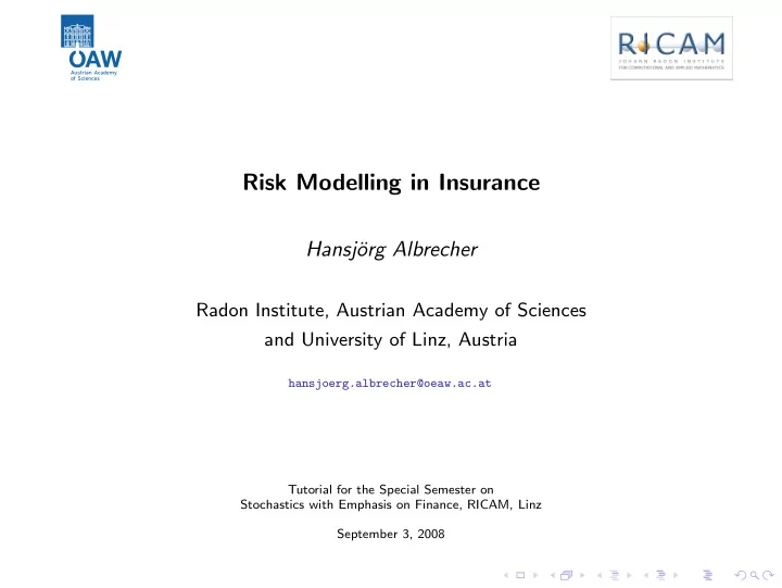
Risk Modelling in Insurance Hansj¨ org Albrecher Radon Institute, Austrian Academy of Sciences and University of Linz, Austria hansjoerg.albrecher@oeaw.ac.at Tutorial for the Special Semester on Stochastics with Emphasis on Finance, RICAM, Linz September 3, 2008

Typical Questions in Insurance ◮ Which risks can be insured? ◮ Determination of fair premiums ◮ Stability of insurance activity

Program ◮ Some Generalities ◮ Aggregate Claim Distributions ◮ Collective Risk Models ◮ Extensions (Dividends, Taxes, Dependence) ◮ Statistical Issues Collection of ideas and approaches, not exhaustive treatment!

Insurance Portfolio Premium Income P ( t ) Claim Payments X 1 + X 2 + · · · + X N ( t ) Initial Capital x Reserve at time t : N ( t ) � R ( t ) = x + P ( t ) − X i i =1 − → Diversification (in the collective, over time,..) Quantitative Approach: Risk Theory (Modelling, Measuring Risk, Control)

Risk Y (random variable) Examples of Measures of Risk ◮ E ( Y ) , Var ( Y ) √ E ( Y ) , skewness S ( Y ) = E (( Y − E ( Y )) 3 ) Var Y ◮ CoV( Y ) = (Var( Y )) 3 / 2 ◮ Value at Risk: VaR α ( Y ) = q α = inf { y | F Y ( y ) ≥ α } − → Capital requirements (Basel II, Solvency II) (normal distribution) ◮ Coherent Risk Measures (Axioms) ◮ Expected Shortfall: � 1 1 ES α ( Y ) = E [ Y | Y > q α ] = α VaR s ds 1 − α (e.g. Swiss Solvency Test)

Crucial: Distribution of Aggregate Claims X ( t ) = � N ( t ) n =1 X n Individual Model � n i =1 X i : ◮ Single payments X i ≥ 0 with F i ( x ) = P ( X i ≤ x ) (policy i ) ◮ X i independent, distribution identical or volume-dependent ◮ Convolutions! � x P ( X 1 + X 2 + .. + X n < x ) := F ∗ n ( x ) = F ∗ ( n − 1) ( x − s ) dF 1 ( s ) 0 � x P ( X 1 + X 2 < x ) = F 2 ( x − s ) dF 1 ( s ) 0 Explicit e.g. for ◮ Gamma distribution: α α µ α Γ( α ) x α − 1 exp( − x α/µ ) , f ( x ) = x > 0 ◮ Inverse Gauss distribution: � µα � � µ/ x ) 2 � � f ( x ) = 2 π x 3 exp − α/ 2( x /µ − , x > 0

Aggregate portfolio usually inhomogeneous! What matters: aggregate claim distribution ◮ Collective Model � N ( t ) i =1 X i , N ( t ) .. claim number, X i iid (d.f. F , “mixed distribution”, reliable estimate) Modelling N (1): e.g. ◮ Poisson distribution: P ( N (1) = n ) = e − λ λ n / n ! , n = 0 , 1 , .. ◮ Mixed Poisson, e.g. negative binomial: � α + n − 1 � p α (1 − p ) n , P ( N (1) = n ) = n = 0 , 1 , .. n

Models for Claim Sizes: Heavy Tails: “Few claims determine aggregate claim size” Candidates: e.g. ◮ (Heavy-Tailed) Weibull: f ( x ) = bx b − 1 exp( − x b ) , x > 0 , 0 < b < 1 . All Moments exist ◮ Lognormal: log X i ∼ N ( µ, σ 2 ) f ( x ) = x − 1 (2 πσ 2 ) − 1 / 2 exp( − (log( x ) − µ ) 2 / (2 σ 2 )) , x > 0 , µ ∈ R , σ 2 > 0 . All Moments exist ◮ Pareto: « α „ b F ( x ) = 1 − , x ≥ b > 0 , α > 0 x resp. Shifted Pareto E ( X β ) < ∞ ⇔ β < α Subexponential Class F ∈ S : P ( X 1 + X 2 + . . . + X n > x ) ∼ n (1 − F ( x )) ∀ n ≥ 2 as x → ∞ .

Aggregate Claims X ( t ) = � N ( t ) n =1 X n , X i iid, independent of N ( t ) � ∞ ˆ F ( s ) := E ( e − sX n ) = 0 e − sx dF ( x ), n =0 p n ( t ) z n with p n ( t ) = P ( N ( t ) = n ) Q t ( z ) := E ( z N ( t ) ) = � ∞ G t ( x ) := P { X ( t ) ≤ x } = � ∞ n =0 p n ( t ) F ∗ n ( x ) ∞ p n ( t )ˆ F n ( s ) = Q t (ˆ E [ e − sX ( t ) ] = � F ( s )) n =0 → Moments of X ( t ): E ( X ( t )) = E ( N ) E ( X n ), Var ( X ( t )) = Var ( N ( t )) E 2 ( X n ) + E ( N ( t )) Var ( X n ), etc.

Approximations for X ( t ) ◮ Moment matching „ « x − E [ X ( t )] ◮ Normal Approximation G t ( x ) ≈ Φ √ Var [ X ( t )] ◮ Shifted Gamma, etc. ◮ Edgeworth approximation, orthogonal polynomials ◮ Discretization of claim sizes → recursive methods (Panjer recursions, FFT etc.) ◮ Asymptotic approximations ◮ Subexponential Claims ◮ Superexponential Claims Also useful in modelling credit risk, operational risk etc.

Asymptotic Approximations of G t ( x ) - Subexponential X n If E ( z N ( t ) ) < ∞ for some z > 1: ∞ X G t ( x ) = P ( X 1 + . . . + X N ( t ) > x ) = P ( N ( t ) = n ) F ∗ n ( x ) n =0 ∞ X ∼ P ( N ( t ) = n ) n F ( x ) = E ( N ( t )) F ( x ) n =0 ◮ Simple! Useful for relevant range of x ? 1.0 � 2.0 upper bound upper bound lower bound 0.8 F ( x ) = x − 3 . 3 , N ∼ Poisson(2), � 2.5 a 1 lower bound 0.6 a 2 a 1 � 3.0 a 3 0.4 a 2 � 3.5 a 3 0.2 � 4.0 10 15 20 25 10 15 20 25 Higher-order Approximations Under suitable conditions a k ( x ) = a 1 ( x ) + P k j =1 A j f ( j ) ( x ) , Improvement in certain parameter ranges.

Asymptotic Approximations of G t ( x ) - Superexponential X n Saddlepoint approximations t κ t ( α ) := log E ( e α S t ) Consider the tilted probability measure P α ( S t ∈ dx ) = E ( e α S t − t κ t ( α ) 1 { S t ∈ dx } ) , Choice of α = α ( x ): E α ( S t ) = t κ ′ t ( α ) = x , As x → ∞ , α approaches right abscissa of convergence α 0 = sup { α : κ t ( α ) < ∞} , given that lim α → α 0 κ ′ t ( α ) = ∞ . Var α ( S t ) = t κ ′′ t ( α ) ! St − x < y → Φ( y ) P α q t κ ′′ t ( α ) e − α ( x ) x + κ t ( α ( x )) = ⇒ 1 − G t ( x ) ∼ as x → ∞ . � 2 π κ ′′ α ( x ) t ( α ( x ))

Asymptotic Approximations of G t ( x ) - Superexponential X n II Z ∞ e −| θ | v { M θ ( x + v ) − M θ ( x ) } dv 1 − G t ( x ) = | θ | e −| θ | x 0 − σ F < θ < 0 with M θ ( x ) := P ∞ n =0 a n F ∗ n θ ( x ) and a n := ˆ F n ( θ ) p n ( t ) 1 s If a ( x ) := a [ x ] ∈ R as x ↑ ∞ : 1 − G t ( x ) ∼ e −| θ | x a ( x , θ ) Appropriate choice of θ ! „ α + n − 1 « ` ´ n . ´ α ` b t Example: Pascal process : p n ( t ) = t + b t + b n ! α 1 F ( θ ) = 1 + b b | θ | Γ( α ) e −| θ | x x α − 1 . ˆ ⇒ 1 − G t ( x ) ∼ | t ˆ t ′ ( θ ) | F

A “Robust” View: Classical Collective Risk Model reserve R t claims ~ F(y) premiums N ( t ) � R t = x + c t − X n n =1 x ruin t time N ( t ). . . homogeneous Poisson process ( λ ) X n . . . iid random variables (d.f. F ) c . . . premium density Ruin Probability ψ ( x , T ) = P ( inf 0 ≤ t ≤ T R t < 0 | R 0 = x )

A “Robust” View: Classical Collective Risk Model reserve R t claims ~ F(y) premiums N ( t ) � R t = u + c t − X n n =1 u ruin t time Generalizations: ◮ more general point processes ◮ inflation, interest on the surplus, dividend and tax payments ◮ investment in financial market, reinsurance ◮ delay in claim settlement, dependency

Solution Methods ◮ Exact Solutions ((P)IDE) Infinite time horizon: CP � x c ∂ψ ∂ x − λ ψ + λ ψ ( x − y ) dF ( y ) + λ (1 − F ( x )) = 0 0 with x →∞ ψ ( x ) = 0. lim � ∞ � n � � λµ 1 − λµ � (1 − F n ∗ ψ ( x ) = I ( x )) , c c n =1 � x with F I ( x ) = 1 0 (1 − F X ( y )) dy , x ≥ 0. µ Examples: c e − c − λµ ◮ X i ∼ Exp(1 /µ ): ψ ( x ) = λµ x c µ ◮ X i ∼ Phase-Type

Solution Methods ◮ Exact Solutions ((P)IDE) Finite time horizon: CP � x c ∂ψ ∂ x − ∂ψ ∂ T − λ ψ + λ ψ ( x − y , T ) dF ( y ) + λ (1 − F ( x )) = 0 0 with x →∞ ψ ( x , T ) = 0 ( T ≥ 0) and ψ ( x , 0) = 0 ( x ≥ 0) lim

Solution Methods ◮ Exact Solutions ((P)IDE) Finite time horizon with positive interest rate: CP Z x ( c + i x ) ∂ψ ∂ x − ∂ψ ∂ T − λ ψ + λ ψ ( x − y , T ) dF ( y ) + λ (1 − F ( x )) = 0 0 with x →∞ ψ ( x , T ) = 0 ( T ≥ 0) and ψ ( x , 0) = 0 ( x ≥ 0) lim i ..real interest force ψ ( x , t ) = a 0 ( t ) + P k E.g. λ = k i , X ∼ Exp ( α ): Gamma Series Expansion n =1 a n ( t )Γ( x ; α, n ) Z u α n y n − 1 e − α y dy with Γ( x ; α, n ) = ( α > 0 , n > 0) Γ( n ) 0 n − 1 ( α x ) j ∂ Γ( x ; α, n ) “ ” Γ( x ; α, n ) = 1 − e − α x X n ∈ N : , = α Γ( x ; α, n − 1) − Γ( x ; α, n ) j ! ∂ x j =0 Recurrence equation 1 “ ( λ + α c − i n ) a n ( t ) + a ′ ” a n +1 ( t ) = n ( t ) + ( i ( n − 1) − λ ) a n − 1 ( t ) α c 1 a ′ a 1 ( t ) = ` 0 ( t ) + λ a 0 ( t ) ´ , a 0 ( t ) = U (0 , t ) α c