
ECO 352 – Spring 2010 No. 6 – Feb. 18 RICARDIAN MODEL CONTINUED EMPIRICAL EVIDENCE Can't expect a literal test of the model; it deliberately leaves out a lot. But can expect evidence about some of its central ideas. [1] Cross-section evidence Wage differences across countries do reflect productivity differences Low-wage “competing” countries also have lower productivity. Figure from K-O p. 43, based on Ashenfelter and Jurajda paper. 1
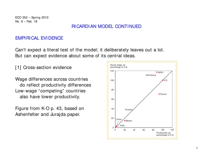
[2] Time-series evidence Wage changes over time reflect productivity changes Figure from Feenstra. These are average labor productivity figures for economy But the productivities in different sectors will be dispersed around this average, and the pattern can vary from one country to another. 2
[3] Bi-lateral export patterns reflect bi-lateral relative productivity differences Picture from Irwin. Bottom line: A country has cost advantage in trade in those sectors where its productivity advantage is greater than its wage disadvantage, or where its wage advantage is greater than its productivity disadvantage 3
MANY TRADED GOODS Label the goods 1, 2, 3, … 19 (say) such that A 1 / A* 1 < A 2 / A* 2 < A 3 / A* 3 < ... < A 19 / A* 19 Assertion: It cannot be true that Home produces a higher-ranked good than Foreign Proof: Assume the opposite; say Home produces 7 and Foreign produces 4. This require P T 7 = A 7 W, P T 4 = A* 4 W* But P T 4 < A 4 W, P T 7 < A* 7 W* , otherwise unexploited profit opportunities These imply A 4 / A 7 > P T 4 / P T 7 > A* 4 / A* 7 , so Therefore A 4 / A* 4 > A 7 / A* 7 . This contradicts the chosen order of labeling. So the opposite assumption must be wrong; the original assertion correct. Conclusion: Home produces an initial range 1, 2, … of goods, Foreign a final range … 17, 18, 19. At most one good in this chain can be produced in both countries. Compare this with the result for the types of equilibria with 2 traded goods, involving complete and incomplete specialization. 4
How to find where the chain breaks? Must “endogenize” wages Use relative labor demand function: (L/L* ) d expressed as function of (W/W* ) Observe that A* 1 / A 1 > A* 2 / A 2 > A* 3 / A 3 > ... > A* 19 / A 19 When W / W* > A* 1 / A 1 , W A 1 > W* A* 1 and then W A 2 > W* A* 2 also. No one wants to produce anything in Home; (L/L* ) d = 0. When W / W* = A* 1 / A 1 , good 1 can be produced at home. But quantity indeterminate therefore (L/L* ) d has a horizontal segment When A* 1 / A 1 > W / W* > A* 2 / A 2 , good 1 produced at Home, 2,... Foreign W/W* s As W drops, price of 1 drops; demand shifts (L/L*) toward it, raising demand for L. And so on. Relative labor demand curve as shown d Its intersection with fixed relative supply (L/L*) determines equilibrium; and therefore the location of production in countries. L/L* Two types of equilibria: on flat, one good in common On downward-sloping part, complete specialization. 5
NON-TRADED GOODS Back to 2 traded goods. Introduce one non-traded good Z. This must be produced in each country to meet local demand. Suppose Home country produces X good, so P T X = W T A X , It also produces the Z good, so P Z = W T A Z . Then P Z / P T X = A Z / A X . Similarly, for Foreign P* Z / P T Y = A* Z / A* Y . Thus price of the non-traded good in each country is tied to the price of the traded good it produces in equilibrium. Implication: In Home country, if A X decreases, P Z / P T X must rise, even though labor in Z remains just as productive as before. Why? This sector must now compete for labor with the X sector that pays higher wage. What happens to the quantities produced? Depends on income elasticity of Z, and substitution between X and Z 6
Historically, many manufactures were traded, services mostly non-traded Labor productivity increased much faster in manufacturing than in services Where this happened more, the country became richer / more developed Implication: More developed countries should have higher prices of services relative to manufactures. The latter are equalized across countries by trade. Therefore more developed countries should have higher overall price levels. This is the Balassa-Samuelson effect, and is observe in data. 7
It is also one reason for departures from purchasing power parity that are captured by The Economist magazine's Big Mac Index 8
ONE MORE LOOK AT ABSOLUTE AND COMPARATIVE ADVANTAGE Effect of technological progress: Suppose a country's productivity in all goods doubles: both A X , A Y are halved. Suppose it (produces and) exports good X W T /P T X = 1/A X is doubled W T /P T Y = ( W T /P T X ) ( P X /P Y ) Of these, W T /P T X doubles. What happens to the “terms of trade” P X /P Y ? The country's export supply will shift out, so its terms of trade may worsen if it is sufficiently large in international trade. In fact we will later see that technology improvement (growth) in a country's export sector may worsen terms of trade so much that it becomes worse off! This is called “immiserizing growth”. But for most countries in reality, the effect on terms of trade is negligible. In the calculation above, W T /P T Y will also nearly double It is broadly correct to say that a uniform increase in productivity will increase the country's living standard in the same proportion. 9
WEAK POINTS OF THE RICARDIAN MODEL [1] Technological differences (labor input coefficients) are simply assumed, How do they persist when technology is a recipe which anyone can use? Possible answer: No; some other skills are required in using recipes. Some countries can't organize production, make and enforce contracts etc. Another possible answer: Labor productivity differences are due to different amounts of other factors, especially capital. Consider correlation between exports and relative productivities across industries in bilateral US-Japan trade. If US has more capital relative to labor, US labor productivity could be higher in all industries, but relatively more so in capital-intensive ones (agriculture!) Then the correlation actually supports quite a different theory: Comparative advantage governed by relative factor endowments. [2] With just one factor mobile across sectors, there is just one wage No distributive conflict. But such conflict is an important aspect of reality. We will next turn to models that cover these aspects. 10
SPECIAL FEATURES OF PREVIOUS MODELS Pure exchange, or all factors specific to uses: [1] Captures very short run [2] PPF is rectangular, supply completely inelastic Ricardian model: one factor, mobile across sectors [1] Captures long run, but no distributive conflict [2] PPF is straight line; supply responds suddenly at one critical relative price Better approach to reality needs some intermediate settings and combinations: [1] Multiple factors with different degrees of mobility across sectors If one US state is hit with a regional shock, unemployment rate falls back to national level within 6 years. In comparison, capital depreciates over 15-20 years, and structures over 30-50 years. (But there may be easier shift of some kinds of workers, equipment, structures across uses.) [2] Regular bowed-out PPF; gradual supply response. The next two models depict such situations Ricardo-Viner: Capital specific to sectors, labor mobile across sectors Heckscher-Ohlin: Both capital and labor mobile across sectors 11
Recommend
More recommend