Topic 1: Dynamics of Credit Ratings, continued Empirical data show - PowerPoint PPT Presentation
Topic 1: Dynamics of Credit Ratings, continued Empirical data show that observed rating transition frequen- cies vary from year to year. Some variation would be expected because of sampling vari- ability, but we must consider the
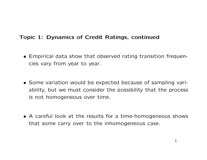
Topic 1: Dynamics of Credit Ratings, continued • Empirical data show that observed rating transition frequen- cies vary from year to year. • Some variation would be expected because of sampling vari- ability, but we must consider the possibility that the process is not homogeneous over time. • A careful look at the results for a time-homogeneous shows that some carry over to the inhomogeneous case. 1
• We now write, for t < u , p i,j ( t, u ) = P [ X ( u ) = j | X ( t ) = i ] , and P ( t, u ) as the matrix with these as entries. • These matrices still satisfy Chapman-Kolmogorov equations: if s < t < u , then P ( s, u ) = P ( s, t ) P ( t, u ) . • In discrete time, one-step transition matrices are also still the key, because repeated use of the Chapman-Kolmogorov equations gives P ( s, u ) = P ( s, s + 1) P ( s + 1 , s + 2) . . . P ( u − 1 , u ) . 2
• Write P t = P ( t, t + 1), the one-year transition matrix for the the time step t → t + 1. • For the entries in P t , write p i,j,t = P [ X ( t + 1) = j | X ( t ) = i ] . • Our problem is to model the dependence of p i,j,t on t . • We assume that we have some covariates z t , and that p i,j,t depends on t only through these covariates; it also depends on a parameter vector θ : p i,j,t = p i,j ( z t ; θ ) . 3
Likelihood Inference • Suppose that we have rating histories for a number of issuers, and wish to estimate θ . • In inference problems generally, the likelihood function is of- ten the starting point. • Suppose that we have rating histories for N issuers for T + 1 time steps: R n ( t ) = rating of n th issuer at time step t, n = 1 , 2 , . . . N ; t = 0 , 1 , . . . , T. 4
n th • For the issuer, the probability of being in rating R ( t + 1) at time t + 1 given being in state R ( t ) at time t is p R n ( t ) ,R n ( t +1) ( z t ; θ ). • By the Markov property, the probability of the history for the n th issuer is therefore T − 1 � p R n ( t ) ,R n ( t +1) ( z t ; θ ) . t =0 • If we assume that transitions for different issuers are inde- pendent, given the covariates z t , the likelihood function is just the product of these issuer-specific probabilities: T − 1 N � � L ( θ ) = p R n ( t ) ,R n ( t +1) ( z t ; θ ) . n =1 t =0 5
• Suppose that N i,j ( t ) issuers make the transition from state i at time t to state j at time t + 1. • Then L ( θ ) contains N i,j ( t ) factors equal to p i,j ( z t ; θ ). • So we can also write T − 1 p i,j ( z t ; θ ) N i,j ( t ) . � � L ( θ ) = t =0 i,j • Since the likelihood depends on the transition histories only through the tables of transition frequencies N i,j ( t ), these are sufficient statistics . 6
• Suppose that θ 1 θ = θ 2 . . . and that p i,j ( z t ; θ ) depends only on the corresponding block θ i . • Then we can also write T − 1 p i,j ( z t ; θ i ) N i,j ( t ) � � � L ( θ ) = t =0 i j � = L i ( θ i ) , i say. 7
• So if we estimate θ by maximizing the likelihood, we can just maximize each term L i ( θ i ) individually. • But T − 1 p i,j ( z t ; θ i ) N i,j ( t ) � � L i ( θ i ) = t =0 j is the same as the likelihood for a multinomial situation: – for t = 0 , 1 , . . . , T − 1, N i ( t ) = � j N i,j ( t ) issuers are ran- domly assigned new ratings j ; – probability of rating j is p i,j ( z t ; θ i ). 8
• So we can use methods for modeling and estimating the probabilities in multinomial situations to model and estimate the Markov Chain transition probabilities. • The most widely used method for binomial data is logistic regression . • The simplest generalization of binomial logistic regression to the multinomial case (with ordered categories such as credit ratings) is cumulative logistic regression. 9
Regression Models for Probabilities • Simplest case: a binary response X and a single covariate z . • Example: Space shuttle O-ring failures: 1 if O-ring shows “thermal distress” on launch; X = 0 otherwise; z = ambient temperature at launch time. • We want to express P [ X = 1] as a function of z . 10
• We could use a linear model: P [ X = 1] = β 0 + β 1 z, but extreme values of z would give “probabilities” either < 0 or > 1, both impossible. • The “odds ratio” P [ X = 1] P [ X = 1] P [ X = 0] = 1 − P [ X = 1] can be any positive value, and its logarithm � � P [ X = 1] log 1 − P [ X = 1] can be any real value. 11
• So the model � � P [ X = 1] log = β 0 + β 1 z 1 − P [ X = 1] always implies a probability between 0 and 1 (exclusive). • Solving for P [ X = 1] gives e β 0 + β 1 z 1 P [ X = 1] = 1 + e β 0 + β 1 z = 1 + e − ( β 0 + β 1 z ) . • This is called a logistic regression model. It is an example of a generalized linear model. 12
• Often we have more than one covariate; the model general- izes to 1 P [ X = 1] = 1 + e − ( β 0 + β 1 z 1 + ··· + β k z k ) 1 = 1 + e − z T β where 1 β 0 z 1 β 1 z = and β = . . . . . . . z k β k • SAS proc logistic will fit this model. 13
• What if X takes more values? Say 0 , 1 , . . . , N − 1 for N > 2. • Two different generalizations for different situations: – If X is an ordinal scale, use cumulative (or ordinal) logistic regression. – If X is a nominal (that is, unordered) scale, use multino- mial logistic regression. • Credit ratings are an ordinal scale, so cumulative logistic regression is the natural choice, but multinomial logistic re- gression could also be used. 14
Cumulative Logistic Regression • For j = 0 , 1 , . . . , N − 1, write 0 X ≤ j X j = 1 X > j. • X j is binary, so we can write a logistic model: � � P [ X j = 1] = z T β j . log 1 − P [ X j = 1] • We have assumed that the same covariates z are relevant to each X j , but we must allow the parameters β j to depend on j . 15
• In the conventional cumulative logistic regression, only the intercept depends on j : β 0 ,j β 1 β j = . . . . β k • In terms of X , we have � � P [ X > j ] = z T β j log P [ X ≤ j ] = β 0 ,j + β 1 z 1 + · · · + β k z k . • SAS proc logistic will fit this model. 16
Motivation for Cumulative Logistic Regression model • Suppose that X is determined by an unobserved continuous variable ξ . • For example, a bond issuer’s credit rating is determined by its underlying financial strength, which does not have to fall into neat categories. • X results from categorizing ξ at N − 1 cut-points x 0 < x 1 < · · · < x N − 2 : X = j ⇐ ⇒ x j − 1 < ξ ≤ x j where we take x − 1 = −∞ and x N − 1 = + ∞ . 17
• Now suppose that ξ is related to the covariates by ξ = β 1 z 1 + · · · + β k z k + ǫ where ǫ has cumulative distribution function F ( · ). • Then � � P [ X ≤ j ] = P ξ ≤ x j � � = P ǫ ≤ x j − β 1 z 1 − · · · − β k z k � � = F x j − β 1 z 1 − · · · − β k z k . 18
• If ǫ has the logistic distribution, that is 1 F ( x ) = 1 + e − x , then � � 1 − F ( x ) log = − x F ( x ) and � � 1 − F x j − β 1 z 1 − · · · − β k z k � � P [ X > j ] log = log � � P [ X ≤ j ] x j − β 1 z 1 − · · · − β k z k F = − x j + β 1 z 1 + · · · + β k z k . • If we write β 0 ,j = − x j , this is the same as the cumulative logistic regression model. 19
• So fitting the cumulative logistic regression model is essen- tially the same as estimating the cut-points x j and the re- gression coefficients β 1 , . . . , β k . • If ǫ is assumed to have the standard normal distribution in- stead of the logistic distribution, we have the cumulative probit regression model. • SAS proc logistic will fit this model. 20
Multinomial Logistic Regression model • For nominal data, the cumulative probabilities modeled in the cumulative logistic regression model have no meaning. • In the Multinomial Logistic Regression model, also known as the Generalized Logistic Regression model, the ratios of the individual probabilities are modeled. • Choose a reference (or base ) category j 0 . Then for j � = j 0 , � � P [ X = j ] = z T β j . log P [ X = j 0 ] 21
• In this model, all elements of β j depend on j : β 0 ,j β 1 ,j β j = . . . . β k,j • Note that the model depends on the choice of the base cat- egory only cosmetically–fitted probabilities are the same, re- gardless of the choice. • SAS proc logistic will fit this model, using the link = glogit option on the model statement. 22
Recommend
More recommend
Explore More Topics
Stay informed with curated content and fresh updates.


