Retaining the Support Vectors Why Retain the Support Vectors? x 2 i - PowerPoint PPT Presentation
Review: Support Vector Machines (SVMs) Start with labeled data-set: 1. { ( x 1 , y 1 ) , ( x 2 , y 2 ) , . . . , ( x n , y n ) } [ i, y i { +1 , 1 } ] Solve constrained quadratic optimization problem: 2. i 1 X X Maximize: W
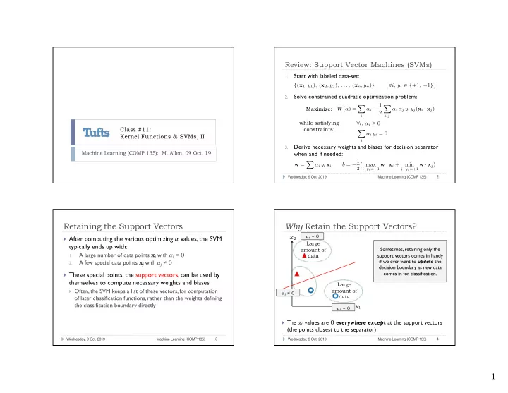
Review: Support Vector Machines (SVMs) Start with labeled data-set: 1. { ( x 1 , y 1 ) , ( x 2 , y 2 ) , . . . , ( x n , y n ) } [ ∀ i, y i ∈ { +1 , − 1 } ] Solve constrained quadratic optimization problem: 2. α i − 1 X X Maximize: W ( α ) = α i α j y i y j ( x i · x j ) 2 i i,j while satisfying ∀ i, α i ≥ 0 Class #11: constraints: X α i y i = 0 Kernel Functions & SVMs, II i Derive necessary weights and biases for decision separator 3. Machine Learning (COMP 135): M. Allen, 09 Oct. 19 when and if needed: b = − 1 X w = 2( max i | y i = − 1 w · x i + j | y j =+1 w · x j ) min α i y i x i i 2 Wednesday, 9 Oct. 2019 Machine Learning (COMP 135) Retaining the Support Vectors Why Retain the Support Vectors? x 2 𝛽 i = 0 } After computing the various optimizing 𝛽 values, the SVM Large typically ends up with: Sometimes, retaining only the amount of A large number of data points x i with 𝛽 i = 0 data support vectors comes in handy 1. if we ever want to update the A few special data points x j with 𝛽 j ≠ 0 2. decision boundary as new data comes in for classification. } These special points, the support vectors, can be used by themselves to compute necessary weights and biases Large } Often, the SVM keeps a list of these vectors, for computation amount of 𝛽 j ≠ 0 data of later classification functions, rather than the weights defining the classification boundary directly x 1 𝛽 i = 0 } The 𝛽 i values are 0 everywhere except at the support vectors (the points closest to the separator) 3 4 Wednesday, 9 Oct. 2019 Machine Learning (COMP 135) Wednesday, 9 Oct. 2019 Machine Learning (COMP 135) 1
<latexit sha1_base64="W/ArN7Cg6WsO2G9XBhHqwZNG8U4=">ACYHicZVFNT+MwEHUCuxTYXVK4wcUCrdRqyrpHhYhIVw4QiIAhLuVo7jtFYdOziTihLlX/C7uHOEX4L7gUTpSJae37wZzyHqRQZ+P6L46sfvu+Vlnf2Pzx89eWV92+znRuGO8wLbW5DWnGpVC8AwIkv0Np0ko+U04PJ3kb0bcZEKrKxinvJvQvhKxYBQs1fOKY0kFAZhXDyUDdLAH7fHso6PMRlRkw7EJ0dExZpWMpM9OT+PqcRrs1zR/NmYXFZ/leYgP5MJPWed+A3/WngZRDMwUF7n/x5emPz3veM4k0yxOugEmaZXeBn0K3oAYEk7zcIHnGU8qGtM+LqTUl/m2pCMfa2KMAT9kFndIwtWKh+i6H+LBbCJXmwBWbtYlzie0KExdxJAxnIMcWUGaEfR+zATWUgfV6oZPJY8aeDT5oMjOKva6gdJy85rDQi+rsMrlvN4G+zdWGdOEGzqKA9tI9qKED/UBudoXPUQy9OmuO51SdN7fibrnVmdR15jU7aCHc3XesRLlj</latexit> Why Retain the Support Vectors? Why Retain the Support Vectors? x 2 𝛽 i = 0 x 2 𝛽 i = 0 Large Large In such scenarios, the data for If the new data remains close to amount of amount of which 𝛽 = 0 before remains that the old boundary, then we can data data way, and never needs to be compute the new 𝛽 - values using reconsidered when solving the only the new data and the (compute-intensive) optimization previous support vectors step of the SVM Large Large 𝛽 j ≠ 0 Only three points have their amount of amount of 𝛽 j ≠ 0 ?? data data 𝛽 - values re-computed x 1 x 1 𝛽 i = 0 𝛽 i = 0 5 6 Wednesday, 9 Oct. 2019 Machine Learning (COMP 135) Wednesday, 9 Oct. 2019 Machine Learning (COMP 135) Why Retain the Support Vectors? Pros and Cons of SVMs } [+] Compared to linear classifiers like logistic regression, SVMs: } Another reason to retain vectors rather than weights is that SVMs are often used with kernel functions that: Are insensitive to outliers in the data (extreme class examples) 1. Transform the data Give a robust boundary for separable classes 1. 2. Compute necessary dot-products of points Can handle high-dimensional data, via transformation 2. 3. ( ϕ : R n → R m ) Can find optimal 𝛽 - values, with no local maxima k ( x , z ) = ϕ ( x ) · ϕ ( z ) 4. } Furthermore, there are some popular such functions where } [–] Compared to linear classifiers like logistic regression, SVMs: the data transform translates n -dimensional to m -dimensional Are less applicable in multi-class ( c > 2 ) instances 1. data with n << m Require more complex tuning, via hyper-parameter selection 2. } In such cases, storing the original n -dimensional data, and then May require some deep thinking or experimentation in order to 3. computing the transformation when necessary, can be much more select the appropriate kernel functions efficient than trying to store the m -dimensional weight information } This is especially true in cases where m = ∞ (!!) 7 8 Wednesday, 9 Oct. 2019 Machine Learning (COMP 135) Wednesday, 9 Oct. 2019 Machine Learning (COMP 135) 2
<latexit sha1_base64="xH/XpF2Y5lr410kQlrN8GKYCiU=">ACMXicZVDLThsxFPVQSiE8GmDJxgJVAqlEM+mibBCo3SDBgkoEkJgw8ng8iYXHuxrBIz8A/0YFvQ/uoYdsOUn6kzCIuVKto6Pz732OWkpuIEwfAwmPkx+nPo0PdOYnZtf+NxcXDo2ymrKOlQJpU9TYpjgknWAg2CnpWakSAU7S9+Du5Prpg2XMkjuClZtyA9yXNOCXgqaR7ElOisGu0FgX6aV9cOb+K3w61zDm/j2FxqGJji6Ti25E7r6TD69cJ9LbhG+ct10ja6FrbAu/B5EI7C2u2+3dmbvfh8mzb9xpqgtmAQqiDFnUVhCtyIaOBXMNWJrWEnoBemxqvbq8BdPZThX2i8JuGbHdFJB7W2s+8xCvtWtuCwtMEmHY3IrMCg8iAVnXDMK4sYDQjX372PaJ5pQ8OGNTdJWsOwrvhoknvm/ip7y+n7RZnUA0f9234Pjdiv61mr/8kn8QMOaRitoFa2jCH1Hu2gPHaIOougePaBn9BL8CR6Dp+BlKJ0IRj3LaKyC13/d3azs</latexit> Gaussian Radial Basis Function (RBF) Gaussian Radial Basis Function k ( x , z ) = e − || x − z || 2 k ( x , z ) = e − || x − z || 2 2 σ 2 2 σ 2 } The RBF is based on a distance from a central focal point, z } The can be measured in a variety of ways, but is often Euclidean: } A popular kernel v with many uses is z n u X u || x − z || = ( x i − z i ) 2 the Gaussian RBF t i =1 Image source: https://www.cs.toronto.edu/~duvenaud/cookbook/ Image source: https://www.cs.toronto.edu/~duvenaud/cookbook/ 9 10 Wednesday, 9 Oct. 2019 Machine Learning (COMP 135) Wednesday, 9 Oct. 2019 Machine Learning (COMP 135) Gaussian Radial Basis Function Gaussian Radial Basis Function k ( x , z ) = e − || x − z || 2 k ( x , z ) = e − || x − z || 2 2 σ 2 2 σ 2 || x − z || = 0 || x − z || → ∞ k ( x , z ) = e 0 = 1 k ( x , z ) → e −∞ = 0 } The value of the } The value drops function is highest to 0 as we get at point z itself further from z Image source: https://www.cs.toronto.edu/~duvenaud/cookbook/ Image source: https://www.cs.toronto.edu/~duvenaud/cookbook/ 11 12 Wednesday, 9 Oct. 2019 Machine Learning (COMP 135) Wednesday, 9 Oct. 2019 Machine Learning (COMP 135) 3
Gaussian Radial Basis Function Gaussian Radial Basis Function k ( x , z ) = e − || x − z || 2 k ( x , z ) = e − || x − z || 2 2 σ 2 2 σ 2 σ → ∞ Tuning Parameter k ( x , z ) → e 0 = 1 } 𝜏 controls the } If 𝜏 gets larger, the diameter of the non-0 area will non-zero area become wider Image source: https://www.cs.toronto.edu/~duvenaud/cookbook/ Image source: https://www.cs.toronto.edu/~duvenaud/cookbook/ 13 14 Wednesday, 9 Oct. 2019 Machine Learning (COMP 135) Wednesday, 9 Oct. 2019 Machine Learning (COMP 135) Gaussian Radial Basis Function Gaussian Radial Basis Function k ( x , z ) = e − || x − z || 2 k ( x , z ) = e − || x − z || 2 x 2 2 σ 2 2 σ 2 σ → 0 k ( x , z ) → e −∞ = 0 x 1 } If 𝜏 gets smaller, non-0 area will } The radius around the focal point z at which the function becomes 0 corresponds to the decision boundary in our data become narrower Image source: https://www.cs.toronto.edu/~duvenaud/cookbook/ 15 16 Wednesday, 9 Oct. 2019 Machine Learning (COMP 135) Wednesday, 9 Oct. 2019 Machine Learning (COMP 135) 4
Gaussian Radial Basis Function Next Week x 2 3 } Topics : SVMs and Feature Engineering e − || x − z j || 2 X k ( x , z 1 , z 2 , z 3 ) = 2 σ 2 } Meetings : Tuesday and Wednesday, usual time j =1 } Readings : Linked from class website schedule page } Includes original paper (Brown, et al.) for discussion } Homework 03 : due Wednesday, 16 October, 9:00 AM } Project 01 : out Tuesday; due Monday, 04 November, 9:00 AM x 1 } Office Hours : 237 Halligan, Tuesday, 11:00 AM – 1:00 PM } We can deal with multiple clusters in the data by using a } TA hours can be found on class website as well combination of multiple RBFs 17 18 Wednesday, 9 Oct. 2019 Machine Learning (COMP 135) Wednesday, 9 Oct. 2019 Machine Learning (COMP 135) 5
Recommend
More recommend
Explore More Topics
Stay informed with curated content and fresh updates.
