Response Surface Methods in Optimization A nonlinear Response - - PowerPoint PPT Presentation

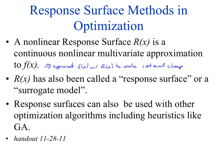
Response Surface Methods in Optimization

• A nonlinear Response Surface R(x) is a

continuous nonlinear multivariate approximation to f(x).

• R(x) has also been called a “response surface” or a

“surrogate model”.

• Response surfaces can also be used with other
• ptimization algorithms including heuristics like

GA.

• handout 11-28-11

Why Use Response Surface approximation Methods?

• A Response Surface approximation R(x) can be

used as part of an efficient parallel optimization algorithm in order to reduce the number of points at which we evaluate f(x), and thereby significantly reduce computational cost.

• Our Response Surface approximation algorithm

searches for the global minimum.

• The term “surrogate” is used to imply that the

response surface is replacing the true function f(x).

Combining Evolutionary Algorithms with Surrogate Response Surface Methodology for Improved Efficiency for Costly Functions

Rommel Regis and Christine Shoemaker

This is a summary (with additional graphs and explanations) of a paper that is in the journal: IEEE Evolutionary Computing (2004) This journal is the second highest cited journal in Computer Science-Artificial Intelligence in the world Web of Science 5 year impact factor: 7.621

Here we talk about application to the “Evolution Strategy” (ES) algorithm.

Initial use of Surrogate Response Surface with Heuristic

• This paper was the first use of a Radial Basis Function

(RBF) with a (meta) heuristic.

• I think it was the first use of any non-quadratic response

surface to a heuristic.

• Heuristics are typically not practical for computationally

expensive functions because they require so many evaluations.

• Surrogate Response surface plus heuristics are a viable

way to solve some global optimization problems with computationally expensive functions.

Experimental Design with Symmetric Latin Hypercube (SLHD)

• To fit the first Response Surface approximation we

need to have evaluated the function at several points.

• We use a symmetric Latin Hypercube (SLHD) to

pick these initial points. (This is a experimental design to distribute points in space evenly- you do not need to know SLHD algorithm.)

• The number of points we evaluate in the SLHD is

(d+1)(d+2)/2, where d is the number of parameters (decision variables).

x (parameter value-one dimensional example) Objective Function f(x) measure of error

One Dimensional Example of Experimental Design to Obtain Initial SurrogateResponse Surface approximation

Costly Function Evaluation (e.g. over .5 hour CPU time for one evaluation).

x (parameters) f(x) Response Surface approximation with Initial Points from Experimental Design In real applications x is multidimensional since there are many parameters (e.g. 10).

x (parameter value) f(x)

Update in Response Surface approximation with New Evaluation

Update done in each iteration for Response Surface approximation for each algorithm expert.

Response Surface approximation is a guess of the function value of f(x) for all x. new

Coupling Response Surface approximation Methods to Heuristic Methods

• Evaluation of the objective function f(x) is

in some cases very COSTLY in CPU time.

• Heuristic Methods tend to require many

function evaluations of f(x) in comparison to other methods.

• We can combine Response Surface

approximation with heuristic methods to improve efficiency.

Response Surface approximation Optimization for Evolutationary Algorithm

• 1. Use a “space filling” experimental design (e.g. SLHD) to

select a limited number of evaluation points.

• 2. Make an approximation of the function (with Radial Basis

Function splines) R(x) based on experimental design

• points. Randomly generate M parents.
• 3. Generate N children from M parents using an evolutionary

algorithm (e.g. Genetic Algorithm or ES).

• 4. Pick the W children {xi} that have the best R(xi).
• 5. Evaluate the real function F(xi) at each of the W children.

Pick the best M of these W children to be the new parents.

• 6. Fit an updated response surface R(x) based on the new

values of F(xi) in 5.) plus all the previously evaluated points.

• 7. Stop if reach maximum number of iterations. Otherwise

go to Step 3

Graph Notation

• ES = evolutionary strategy
• ES plus is

– SLHD=with symmetric hypercube initially – QR= response surface by quadratic approximation and initial SLHD – RBF=response surface with radial basis function (RBF) and initial SLHD

Notation in Graphics results

• ESRBF (10, 8, 50, 20)—means you have

– M=8 parents, – you generate N=50 offspring that are evaluated by the response surface R(x) – You evaluate expensive function F(x) the best W= 20 based on R(x) – You pick the best M=8 to be the parents based on the values of F(x) The first number (10) relates to the size of the SLHD so you can ignore it. M, N, W

Variables in Graphs: (M,W)-ES (no response sur) (SLHD, M,N,W) for ES RBF or ESQR

• 1. Use a “space filling” experimental design (e.g. SLHD)

to select a limited number of evaluation points.

• 2. Make an approximation of the function (with Radial Basis

Function splines) R(x) based on experimental design

• points. Randomly generate M parents.
• 3. Generate N children from M parents using an

evolutionary algorithm (e.g. Genetic Algorithm).

• 4. Pick the W children {xi} that have the best R(xi).
• 5. Evaluate the real function F(xi) at each of the W
• children. Pick the best M of these W children to be the

new parents.

• 6. Fit an updated response surface R(x) based on the new

values of F(xi) in 5.) plus all the previously evaluated points.

• 7. Stop if reach maximum number of iterations.

Otherwise go to Step 3

Summary on Response Surface approximation Optimization for Costly Functions

• Response Surface approximation methods

have potential to reduce computational effort significantly for application of heuristics to

• ptimization of continuous functions where

function evaluation is “costly”.

• There are several existing approaches to the

use of response methods. Initial results indicate our new methods are good both in serial and in parallel.

Parallel Optimization

• A major focus of our research is on using response

surface methods for optimization of costly functions in parallel.

• Especially when combined with parallelized costly

function evaluation, parallel optimization can lead to efficient use of a large number of processors.

• This algorithm is the focus of a second NSF grant

(from the Computer and Information Science Directorate) on parallel optimization.

Cornell Univ.: Wild and Shoemaker 16

: , φ

+ →

° °

( )

( )

( )

2 1

,

k k j j j

m x s s y p s

γ

λ φ

=

+ = − +

∑

( ) ( )

1 1

,

q n i i d i

p s v s π ρ −

=

= ∈

∑

Our Response surface is based on Radial Basis Functions:

a univariate function

a “polynomial tail”. model The yj = F(xj ) are points for which the value of F is known. s is any point on the response surface. Everything else is given or computed.

x (parameter value) f(x)

One Dimensional Response Surface

Response Surface approximation is a guess of the function value of f(x) for all x. new

Cornell Univ.: Wild and Shoemaker 18

Two Dimensional Example: Cubic RBF Surrogate Based on 6 points

( )

8 3 1 2 1 3 2 2 1

,

k j j j

m x s s y v v s v s λ

=

+ = − + + +

∑

cubic

Cornell Univ.: Wild and Shoemaker 19

Two Dimensional Example: Gaussian RBF Surrogate

( )

8 2 2 1 2 1 3 2 1

,

j

s y k j j

m x s e v v s v s λ

− =

+ = + + +

∑

Gaussian

Cornell Univ.: Wild and Shoemaker 20

( )

8 2 1 2 1 3 2, 2 1

1

k j j j

m x s s y v v s v s λ

=

+ = − + − + + +

∑

Example: Multiquadric RBF Surrogate

Multiquadric

Cornell Univ.: Wild and Shoemaker 21

Why Do We Like RBFs?

• 1. Radial Basis Functions (RBF) offer a nonlinear

interpolation model with a linear (in n) number of function evaluations

• 2. Attractive theoretical and numerical properties
• 3. Works well with scattered data (e.g. points computed in

iterative searches of optimization algorithm

• 4. We can add previously evaluated points to the trust

region calculation since RBF is more flexible about location of points than a quadratic model.

Methodoloby

• Pick an evolutionary algorithm, e.g. GA, ES,

DDS.

• To evaluate the cost function f(x) for a population
• f size, get an approximation of f(x) by using the

value of the response surface RS(x).

• Based on the RS(x) values, evaluate the function f

(x) (costly evaluations) at a subset A of the Pmax

• points. A is the set of the M points that have the

best RS(x) values.

• Use the points in A to produce the offspring. For

GA, this means that selection of parents and crossover and mutation is only on the elements of A that have had costly function evaluations

Local Response Surface Approximation

• In this evolutionary application we will use

a local approximation that is based on a fixed number of the closest points around the function value being estimated.

• In other applications we try to approximate

the entire surface using all the points or try to build a mathematically defined “trust region”

Notation

• (µ,λ)-ES– is an evolutionary strategy that

has µ parents and generates λ children that.

• (m,µ,λ,v)-ES is an evolutionary strategy that

has µ parents and generates λ children of which only v will be evaluated by costly function evaluation.

• m is the number of points used in a

symmetric latin hypercube design.

• (ES has a sophisticated strategy for doing

mutations to generate the children, which we won’t discuss here.)

Continutation of Methodology

• Generate an updated Response Surface by

combining the previous computed values of f(x) with the newly computed values of f(x) and fitting the surface.

• Use the current M members of the population to

generate Pmax offspring.

• Repeat previous steps by now picking the best M
• ffspring based on the updated RS(x) values from

the PMAX members of the population.

Psuedo Code for ESGRBF

• 1. Generate experimental design points (SLHD)

and denote this set of points by Ei .

• 2. Evaluate the objective function at the points in

E

• 3. Set t=0
• 4. Set P(t) to be the subset of points in E with the

lowest function values

• 5. Evaluate the Objective Function at the points in

P(t)

Psuedo Code continued

• 6. While not terminate do
• a. P” (t) =mutate P(t) (could also do crossover if desired)
• b. estimate the value of each element of P”(t) from local

response surface approximation using the k=(d+1)(d+2)/2 nearest previously evaluated points.

• c. P”’(t) is defined to be the set of points in P”(t) with the v

best values based on the local response surface.

• d. Evaluate (expensive function simulation) at all the

points in P”’(t)

• e. P(t+1) is the union of P”’(t) and the set of elite parents.
• f. t is updated to be t+1

end

Finite Difference Mesh for Groundwater Problem The problem here is to compute the cheapest way to inject water and substrate to degrade contaminant at groundwater monitoring wells

• ver time with flowing water and contaminant (similar to video)

Groundwater Bioremediation Problem, m=91 (Fig. 4)

Plot is in terms of Numbers of Function Evaluations- Why?

• The cost to do the optimization calculations

including building the surfaces is relatively small (e.g. seconds or about a minute).

• The cost to do the (simulation model) evaluations

is assumed to be large (e.g. many minutes or hours or maybe even days.

• Hence to evaluate the methods for

computationally expensive problems we are primarily interested in evaluation numbers.