resonant response in nonequilibrium stationary states

play

Resonant Response in Nonequilibrium Stationary States Ral - PowerPoint PPT Presentation

Oct 03, 2023 •310 likes •851 views

Introduction Resonant Response Conclusions Resonant Response in Nonequilibrium Stationary States Ral Salgado-Garca Department of physics, Facultad de Ciencias Universidad Autnoma del Estado de Morelos 6th International Workshop on Non

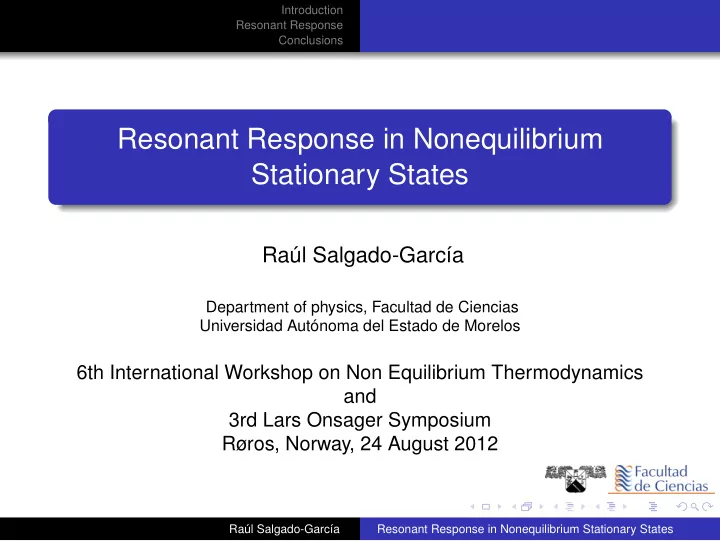
Introduction Resonant Response Conclusions Resonant Response in Nonequilibrium Stationary States Raúl Salgado-García Department of physics, Facultad de Ciencias Universidad Autónoma del Estado de Morelos 6th International Workshop on Non Equilibrium Thermodynamics and 3rd Lars Onsager Symposium Røros, Norway, 24 August 2012 , Raúl Salgado-García Resonant Response in Nonequilibrium Stationary States
Introduction Resonant Response Conclusions Outline Introduction 1 Stationary States Linear Response Resonant Response 2 Linear Response for NESS Relaxation–Response Relation Conclusions 3 , Raúl Salgado-García Resonant Response in Nonequilibrium Stationary States
Introduction Satationary States Resonant Response Linear Response Conclusions Markov Process H = P 2 2 m + V ( x ) + interactions , → dx dt = f ( x ) + ξ ( t ) , � ξ ( t ) ξ ( t ′ ) � = 2 βδ ( t − t ′ ) � ξ ( t ) � = 0 , , Raúl Salgado-García Resonant Response in Nonequilibrium Stationary States
Introduction Satationary States Resonant Response Linear Response Conclusions Markov Process H = P 2 2 m + V ( x ) + interactions , → dx dt = f ( x ) + ξ ( t ) , � ξ ( t ) ξ ( t ′ ) � = 2 βδ ( t − t ′ ) � ξ ( t ) � = 0 , , Raúl Salgado-García Resonant Response in Nonequilibrium Stationary States
Introduction Satationary States Resonant Response Linear Response Conclusions Markov Process H = P 2 2 m + V ( x ) + interactions , → dx dt = f ( x ) + ξ ( t ) , � ξ ( t ) ξ ( t ′ ) � = 2 βδ ( t − t ′ ) � ξ ( t ) � = 0 , , Raúl Salgado-García Resonant Response in Nonequilibrium Stationary States
Introduction Satationary States Resonant Response Linear Response Conclusions Stationary States Statistical description : probability density ρ ( x , t ) L ρ = ∂ t ρ The observables: e. g. Particle current � j ( t ) = � v � = v ( x , t ) ρ ( x , t ) dx Stationary state: t → ∞ ⇒ ρ ( x , t ) → P ss L P ss = 0 , , Raúl Salgado-García Resonant Response in Nonequilibrium Stationary States
Introduction Satationary States Resonant Response Linear Response Conclusions Stationary States Statistical description : probability density ρ ( x , t ) L ρ = ∂ t ρ The observables: e. g. Particle current � j ( t ) = � v � = v ( x , t ) ρ ( x , t ) dx Stationary state: t → ∞ ⇒ ρ ( x , t ) → P ss L P ss = 0 , , Raúl Salgado-García Resonant Response in Nonequilibrium Stationary States
Introduction Satationary States Resonant Response Linear Response Conclusions Stationary States Statistical description : probability density ρ ( x , t ) L ρ = ∂ t ρ The observables: e. g. Particle current � j ( t ) = � v � = v ( x , t ) ρ ( x , t ) dx Stationary state: t → ∞ ⇒ ρ ( x , t ) → P ss L P ss = 0 , , Raúl Salgado-García Resonant Response in Nonequilibrium Stationary States
Introduction Satationary States Resonant Response Linear Response Conclusions Stationary States Statistical description : probability density ρ ( x , t ) L ρ = ∂ t ρ The observables: e. g. Particle current � j ( t ) = � v � = v ( x , t ) ρ ( x , t ) dx Stationary state: t → ∞ ⇒ ρ ( x , t ) → P ss L P ss = 0 , , Raúl Salgado-García Resonant Response in Nonequilibrium Stationary States
Introduction Satationary States Resonant Response Linear Response Conclusions Stationary States Statistical description : probability density ρ ( x , t ) L ρ = ∂ t ρ The observables: e. g. Particle current � j ( t ) = � v � = v ( x , t ) ρ ( x , t ) dx Stationary state: t → ∞ ⇒ ρ ( x , t ) → P ss L P ss = 0 , , Raúl Salgado-García Resonant Response in Nonequilibrium Stationary States
Introduction Satationary States Resonant Response Linear Response Conclusions Equilibrium stationary states (ESS) Once the system has reached the stationary state, can we determine whether a system is in equilibrium or not? Detailed balance P ( x , t | x ′ , t ′ ) ρ ss ( x ′ ) = P ( x ′ , t | x , t ′ ) ρ ss ( x ) , Raúl Salgado-García Resonant Response in Nonequilibrium Stationary States
Introduction Satationary States Resonant Response Linear Response Conclusions Equilibrium stationary states (ESS) Once the system has reached the stationary state, can we determine whether a system is in equilibrium or not? Detailed balance P ( x , t | x ′ , t ′ ) ρ ss ( x ′ ) = P ( x ′ , t | x , t ′ ) ρ ss ( x ) , Raúl Salgado-García Resonant Response in Nonequilibrium Stationary States
Introduction Satationary States Resonant Response Linear Response Conclusions Non-Equilibrium Stationary States (NESS) A NESS does not fulfill the detailed balance condition. Generally, the fluxes in a NESS are not zero. , Raúl Salgado-García Resonant Response in Nonequilibrium Stationary States
Introduction Satationary States Resonant Response Linear Response Conclusions Non-Equilibrium Stationary States (NESS) A NESS does not fulfill the detailed balance condition. Generally, the fluxes in a NESS are not zero. , Raúl Salgado-García Resonant Response in Nonequilibrium Stationary States
Introduction Satationary States Resonant Response Linear Response Conclusions Linear response ∂ρ p ∂ t = L ρ p + ε e i ω t L p ρ p ρ p ≈ P ss + ε e i ω t R , R = Response function ( L − i ω ) R = L p P ss If we know R we can calculate the response for observables j p = j ss + εµ ( ω ) , Raúl Salgado-García Resonant Response in Nonequilibrium Stationary States
Introduction Satationary States Resonant Response Linear Response Conclusions Linear response ∂ρ p ∂ t = L ρ p + ε e i ω t L p ρ p ρ p ≈ P ss + ε e i ω t R , R = Response function ( L − i ω ) R = L p P ss If we know R we can calculate the response for observables j p = j ss + εµ ( ω ) , Raúl Salgado-García Resonant Response in Nonequilibrium Stationary States
Introduction Satationary States Resonant Response Linear Response Conclusions Linear response ∂ρ p ∂ t = L ρ p + ε e i ω t L p ρ p ρ p ≈ P ss + ε e i ω t R , R = Response function ( L − i ω ) R = L p P ss If we know R we can calculate the response for observables j p = j ss + εµ ( ω ) , Raúl Salgado-García Resonant Response in Nonequilibrium Stationary States
Introduction Satationary States Resonant Response Linear Response Conclusions Linear response ∂ρ p ∂ t = L ρ p + ε e i ω t L p ρ p ρ p ≈ P ss + ε e i ω t R , R = Response function ( L − i ω ) R = L p P ss If we know R we can calculate the response for observables j p = j ss + εµ ( ω ) , Raúl Salgado-García Resonant Response in Nonequilibrium Stationary States
Introduction Satationary States Resonant Response Linear Response Conclusions Einstein Relation and Kubo Formula Is P ss is a ESS, Einstein Relation: for ω = 0 � ∞ µ = β D = � v ( t 0 ) v ( t 0 + τ ) � d τ, D = Diffusion coefficient 0 Kubo’s Formula � ∞ � v ( t 0 ) v ( t 0 + τ ) � e i ωτ d τ, µ ( ω ) = 0 The Fluctuation-Dissipation Theorem , R. Kubo, Rep. Prog. Phys. 29 , 255 (1966). , Raúl Salgado-García Resonant Response in Nonequilibrium Stationary States
Introduction Satationary States Resonant Response Linear Response Conclusions Einstein Relation and Kubo Formula Is P ss is a ESS, Einstein Relation: for ω = 0 � ∞ µ = β D = � v ( t 0 ) v ( t 0 + τ ) � d τ, D = Diffusion coefficient 0 Kubo’s Formula � ∞ � v ( t 0 ) v ( t 0 + τ ) � e i ωτ d τ, µ ( ω ) = 0 The Fluctuation-Dissipation Theorem , R. Kubo, Rep. Prog. Phys. 29 , 255 (1966). , Raúl Salgado-García Resonant Response in Nonequilibrium Stationary States
Introduction Linear Response for NESS Resonant Response Relaxation–Response Relation Conclusions Resonant Response R = ( i ω − L ) − 1 L p P ss . ( L − i ω ) R = L p P ss ⇒ For Re [ s ] < 0 � ∞ ( s − L ) − 1 = dt e st e t L 0 We obtain ( s = − δ + i ω ) � ∞ dt e st e t L L p P ss . R = lim δ → 0 + 0 , Raúl Salgado-García Resonant Response in Nonequilibrium Stationary States
Introduction Linear Response for NESS Resonant Response Relaxation–Response Relation Conclusions Resonant Response R = ( i ω − L ) − 1 L p P ss . ( L − i ω ) R = L p P ss ⇒ For Re [ s ] < 0 � ∞ ( s − L ) − 1 = dt e st e t L 0 We obtain ( s = − δ + i ω ) � ∞ dt e st e t L L p P ss . R = lim δ → 0 + 0 , Raúl Salgado-García Resonant Response in Nonequilibrium Stationary States
Introduction Linear Response for NESS Resonant Response Relaxation–Response Relation Conclusions Resonant Response R = ( i ω − L ) − 1 L p P ss . ( L − i ω ) R = L p P ss ⇒ For Re [ s ] < 0 � ∞ ( s − L ) − 1 = dt e st e t L 0 We obtain ( s = − δ + i ω ) � ∞ dt e st e t L L p P ss . R = lim δ → 0 + 0 , Raúl Salgado-García Resonant Response in Nonequilibrium Stationary States
Introduction Linear Response for NESS Resonant Response Relaxation–Response Relation Conclusions Resonant Response By normalization we have that e t L L p P ss = � c λ e λ t P λ λ � = 0 where { P λ } λ is complete basis of eigenfunctions for L , with L P λ = λ P λ , λ = 0 ⇒ P 0 = P ss The we obtain C λ P λ � R = i ω − λ λ � = 0 , Raúl Salgado-García Resonant Response in Nonequilibrium Stationary States

Download Presentation

Download Policy: The content available on the website is offered to you 'AS IS' for your personal information and use only. It cannot be commercialized, licensed, or distributed on other websites without prior consent from the author. To download a presentation, simply click this link. If you encounter any difficulties during the download process, it's possible that the publisher has removed the file from their server.

Recommend

More recommend