Derivation of the GENERIC form of nonequilibrium thermodynamics from - PowerPoint PPT Presentation
Derivation of the GENERIC form of nonequilibrium thermodynamics from a statistical optimization principle Bruce Turkington Univ. of Massachusetts Amherst An optimization principle for deriving nonequilibrium statistical models of Hamiltonian
Derivation of the GENERIC form of nonequilibrium thermodynamics from a statistical optimization principle Bruce Turkington Univ. of Massachusetts Amherst “An optimization principle for deriving nonequilibrium statistical models of Hamiltonian dynamics.” arXiv 1207.2692 “A nonequilibrium statistical model of spectrally truncated Burgers-Hopf dynamics.” (with Richard Kleeman) arXiv 1206.6545 “Best-fit quasi-equilibrium ensembles: a general approach to statistical closure of underresolved Hamiltonian dynamics.” (with Petr Plechac) arXiv 1010.4362
Nonequilibrium thermodynamics is conceived in a general sense as a statistical closure of a complex dynamical system. • A set of resolved (relevant, macroscopic, slow) variables is identified. • All unresolved (irrelevant, microscopic, fast) variables are described by a statistical (probabilistic, stochastic) model. • A closed reduced dynamics approximates (estimates, predicts) the expected (mean, average) evolution of the resolved variables. The approach discussed in this lecture uses 1. An underlying dynamics that is Hamiltonian with n degrees of freedom. 2. Any independent set of m resolved variables; typically, m ≪ n . 3. Canonical statistical models of the unresolved fluctuations. 4. An optimization principle to construct the closed reduced equations. Key idea: The reduced model finds the best fit of all feasible evolutions of the resolved variables to the underlying dynamics.
Dynamical system and statistical model The microstate is a point z = ( q 1 , p 1 , . . . , q n , p n ) ∈ Γ = R 2 n . The microscopic dynamics is canonical Hamiltonian : dq j dp j dt = ∂H dt = − ∂H , . ∂p j ∂q j Every dynamical variable F : Γ → R evolves under dF ∂F ∂H − ∂F ∂H � dt = { F, H } = ∂q j ∂p j ∂p j ∂q j j Examples of interest for reduction: 1. A few heavy particles coupled to a “bath” of many light particles. 2. A set of wave modes in a nonlinear wave system interacting with a “fluctuating” wave field. 3. A large-scale coherent structure immersed in a “background” of small-scale turbulent fluctuations. Sometimes a non-canonical Hamiltonian structure is convenient.
An ensemble of microscopic trajectories, z ( t ), is described by a probability density, ρ ( z, t ), governed by Liouville’s equation : ∂ρ ∂t + Lρ = 0 , with L · = { · , H } For every dynamical variable F , d � F | ρ � . � dt � F | ρ ( · , t ) � = � LF | ρ ( · , t ) � ; = Γ F ( z ) ρ ( z ) dz . But the exact solution, ρ ( t ) = e − tL ρ (0), is not really useful, being too intricate to analyze and too expensive to compute. Instead impose an approximation to ρ ( z, t ) that is parametrized by the statistical averages of some selected resolved variables A = ( A 1 , . . . , A m ) ( each A i : Γ → R )
Canonical statistical model A natural choice of (nonequilibrium) trial probability densities is the parametric family ρ ( z, λ ) = exp[ λ ∗ A ( z ) − φ ( λ )] ρ eq ( z ) ˜ where � Γ exp( λ ∗ A ( z )) ρ eq ( z ) dz λ ∈ R m φ ( λ ) = log for ρ eq is a fixed equilibrium density on Γ; that is, Lρ eq = 0. For instance, ρ eq ( z ) = Z ( β ) − 1 exp( − βH ( z )) [Gibbs canonical ensemble]. λ = ( λ 1 , . . . , λ m ) is the parameter vector for model. Here and throughout, λ ∗ A = λ 1 A 1 + . . . + λ m A m .
ρ ( z, λ ) = exp[ λ ∗ A ( z ) − φ ( λ )] ρ eq ( z ) Two interpretations of ˜ Statistics: ˜ ρ defines a parametric statistical model; specifically, an exponential family with natural parameter λ . The vector A of resolved variables is a minimal sufficient statistic for this parametric model. Physics: Each ˜ ρ is a quasi-equilibrium/canonical ensemble . It maximizes (relative) entropy S ( ρ ) = − � log ρ | ρ � ρ eq subject to the expected value of the vector of resolved variables � A | ρ � = a , � 1 | ρ � = 1 . The entropy function for this model is s ( a ) = S (˜ ρ ( · , λ )) and there is a one-to-one correspondence between a and λ : a = ∂φ λ = − ∂s ∂λ , [Legendre transform] . ∂a
Adiabatic closure A naive way to evolve the parameter λ ( t ) ∈ R m is to impose A 1 , . . . , A m moments of the Liouville equation exactly: d Γ A ( ∂ � dt � A | ˜ ρ � − � LA | ˜ ρ � = ∂t + L ) ˜ ρ dz = 0 . But this closed reduced dynamics is reversible : d dt S (˜ ρ ) = 0 [ entropy is conserved ] This memoryless closure neglects the influence of the unresolved fluctuations on the evolution of the resolved variables. Statistical physicists (Zubarev 1970s and others) advocate using “nonequilibrium statistical operators” with decaying memory �� + ∞ � λ ( t − τ ) e τ ( L − α ) A αdτ − ψ [ λ ]( t ) ρ ( t ) = exp ρ eq 0
Best-fit closure – a different approach Retain the quasi-equilibrium trial densities, and evaluate their Liouville residual along any feasible parameter path λ ( t ): = ( ∂ R . λ ( t ) ∗ ( A − a ( t )) + λ ( t ) ∗ LA ρ ( λ ( t )) = ˙ ∂t + L ) log ˜ The ensemble-averaged evolution of any dynamical variable F along such a path of trial densities: d dt � F | ˜ ρ ( λ ( t )) � − � LF | ˜ ρ ( λ ( t )) � = � FR | ˜ ρ ( λ ( t )) � The statistic R = R ( z ; λ, ˙ λ ) represents the rate of information loss locally at state λ and velocity ˙ λ : At any sample microstate z ∈ Γ, the information for discriminating between the exact density and the trial density after a time increment ∆ t is: log e − (∆ t ) L ˜ ρ ( z, λ ( t )) λ ( t )) + O ( (∆ t ) 2 ) ρ ( z, λ ( t + ∆ t )) = − (∆ t ) R ( z ; λ ( t ) , ˙ as ∆ t → 0 . ˜
Closure concept: Find paths λ ( t ) in the statistical parameter space that are “best-fit” to the Liouville equation in the sense that they minimize R in some time-integrated norm. Separate R into its orthogonal components along the resolved and unresolved subspaces of L 2 (Γ , ˜ ρ ( λ )): R ( λ, ˙ λ ) = P λ R + Q λ R , where λ − C ( λ ) − 1 f ( λ ) ] ∗ ( A − a ) , [ ˙ P λ R = λ ∗ ( Q λ LA ) Q λ R = C ij ( λ ) = � ( A i − a i )( A j − a j ) | ˜ ρ ( λ ) � [Fisher information matrix]. f i ( λ ) = � LA i | ˜ ρ ( λ ) � [Reversible term in flux]. The lack-of-fit cost function : λ ) = � ( P λ R ) 2 | ˜ ρ ( λ ) � + � ( W λ Q λ R ) 2 | ˜ 2 L ( λ, ˙ ρ ( λ ) � . The bounded linear operator W λ on L 2 (Γ) weights the unresolved component Q λ R relative to the resolved component P λ R . W λ contains all the adjustable parameters in the closure.
The best-fit closure minimizes the lack-of-fit cost functional over all feasible parameter paths λ ( t ) , 0 ≤ t < + ∞ : � + ∞ L ( λ, ˙ Minimize λ ) dt over paths λ ( t ) with λ (0) = λ 0 . 0 The initial state λ 0 � = 0 is specified at time t = 0. The predicted (estimated) macrostate at each time t > 0 corresponds to the extremal parameter vector ˆ λ ( t ). The predicted evolution ˆ λ ( t ) represents a relaxation from the nonequilibrium state λ 0 � = 0 towards equilibrium λ eq = 0. ρ ( · , ˆ The evolving trial probability density ˜ λ ( t )) is the best-fit estimate of the true density ρ ( t ) = e − tL ˜ ρ ( λ 0 ) .
The closed reduced equations Introduce the value function (principal function or “action”) of Hamilton-Jacobi theory: � + ∞ L ( λ, ˙ v ( λ 0 ) = min λ ) dt , λ (0)= λ 0 0 which assigns an optimal lack-of-fit to every state λ 0 ∈ R m . v ( λ ) solves the (stationary) Hamilton-Jacobi equation λ, − ∂v � � H = 0 , ∂λ where H ( λ, µ ) is the Legendre transform of L ( λ, ˙ λ ): µ = ∂ L λ = C ( λ )˙ λ − f ( λ ) ∂ ˙ λ ∗ µ − L = 1 2 µ ∗ C ( λ ) − 1 µ + f ( λ ) ∗ C ( λ ) − 1 µ − 1 2 λ ∗ D ( λ ) λ H = ˙ and D ij ( λ ) = � ( W λ Q λ LA i )( W λ Q λ LA j ) | ˜ ρ ( λ ) � .
Along an extremal ˆ λ ( t ) the corresponding ˆ µ ( t ) satisfies µ ( t ) = − ∂v ∂λ (ˆ ˆ λ ( t )) . Replacing µ by its expression in terms of ˙ λ and λ produces the closed reduced equations (first-order DEs in t ): λ ) d ˆ d ˆ a λ λ ) − ∂v λ = − ∂s dt = C (ˆ dt = f (ˆ ∂λ (ˆ ˆ λ ) , with ∂a (ˆ a ) . Recall that C ( λ ) = � ( A − a )( A − a ) ∗ | ˜ a = � A | ˜ ρ ( λ ) � , ρ ( λ ) � , f ( λ ) = � LA | ˜ ρ ( λ ) � . Physical interpretation of canonically conjugate λ and µ : − λ i is the thermodynamic force (affinity) associated with A i . µ i = − ∂v ∂λ i is the corresponding thermodynamic flux . i λ i ∂v i λ i µ i = � − � ∂λ i is the entropy production .
Relation to GENERIC Nonequilibrium Thermodynamics Various authors (Morrison, Beris and Edwards, Grmela and ¨ Ottinger, and others) have proposed a generic format for nonequilibrium macrodynamics: da dt = L ( a ) ∂E ∂a + M ( a ) ∂S ∂a where E = energy , S = entropy , L = − L ∗ , M = M ∗ ≥ 0 . The first term is reversible, a generalized Hamiltonian vector field. The second term is irreversible, a generalized gradient vector field. Our statistical optimization principle produces expressions for these reversible and irreversible terms: ∂E ∂a = ∂h L ( a ) = � { A, A ∗ } � , ∂a ( s, a ) with h ( s, a ) = � H � . M ( a ) ∂S ∂a = − ∂v ∂λ .
Recommend
More recommend
Explore More Topics
Stay informed with curated content and fresh updates.
