Research of short- -term forecast errors term forecast errors - PowerPoint PPT Presentation

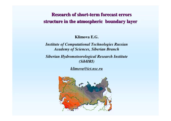
Research of short- -term forecast errors term forecast errors Research of short structure in the atmospheric boundary layer structure in the atmospheric boundary layer Klimova E.G. Institute of Computational Technologies Russian Academy of Sciences, Siberian Branch Siberian Hydrometeorological Research Institute (SibHRI) klimova@ict.nsc.ru

Work is in part supported by the Project on development of Work is in part supported by the Project on development of variational data assimilation system data assimilation system variational (Russian Hydrometeorological Hydrometeorological Center, Moscow). Center, Moscow). (Russian Klimova E.G. , Kilanova N.V., Dubrovskaya O.A. - Institute of Computational Technologies Russian Academy of Sciences, Siberian Branch Siberian Hydrometeorological Research Institute (SibHRI ) Zaripov R. - Russian Hydrometeorological Center, Moskow

The purpose of work: an estimation of the short- -term forecast term forecast The purpose of work: an estimation of the short errors in atmospheric boundary layer boundary layer errors in atmospheric The basic problems: • a large volume of the surface observations; • dependence of correlation of surface forecast errors and forecast errors at the top levels from stability of an atmospheric PBL; • influence of orography.

Data assimilation a algorithms lgorithms: : Data assimilation Kalman filter filter Kalman = f a x A x ; − − k k 1 k 1 = + f a T P A P A Q − − − − k k 1 k 1 k 1 k 1; = + − f T f T 1 K P M ( M P M R ) ; k k k k k k k = − a f P ( I K M ) P ; k k k k = + − a f 0 f x x K ( y M x ); k k k k k k = k 0,..., K . = − − = − − f f t f t T a a t a t T P E x ( x )( x x ) ; P E x ( x )( x x ) . k k k k k k k k k k

Data assimilation algorithms lgorithms: : Data assimilation a 4DVAR 4DVAR ∑ 1 = i n − = − − + T 1 min ( ) ( ( ( ))) ( ( ( ))) J x y H M x O y H M x 0 i i i 0 i i i i 0 = 2 i 0 1 − + − − T 1 ( x x ) P ( x x ) 0 0 b b b 2 − ″ ′ 1 = − × x x J J a b x x b b

Observational data analyses: Observational data analyses: = + − x x K y ( Mx ), a fg 0 fg = + − T T 1 K PM ( MPM O ) , = + ε y Mx 0 fg 0, T = ε ε = ε ε - random m-vector of the E 0 , E ( )( ) O 0 0 0 0 observational errors , P – covariance matrix of the forecast errors. If to assume homogeneity and isotropy of the forecast errors, covariance approximately it is possible to describe as: = σ 2 P F ( 12 r ) 12 f

: Observational data analyses : Observational data analyses ∑ ~ = + − a f o f x x w ( y x ) - interpolation to the grid point k k ik i i i Cov ( i , k ) = w - the weight function + ik 2 ( Cov ( i , i ) r ) pn = σ ρ 2 Cov ( i , k ) F ( ) ik p2 Lf p1 ps

Methods of the forecast error covariance estimation : Methods of the forecast error covariance estimation : • NMC-method; •innovations; •ensemble of forecasts.

Forecast error covariance estimation : Forecast error covariance estimation : • The forecast errors are estimated by the “innovation” vector : = − r ( y Mx ) 0 fg • The “innovations” covariance: T = + T rr MPM R P – forecast error covariance matrix, R – observations error covariance matrix. = 2 2 2 Usually assume, that R diag { r , r , , r } L 1 2 n

Forecast errors covariance estimation : Forecast errors covariance estimation : For forecast error covariance estimation we use: For forecast error covariance estimation we use: • Observations for June - August 2006 (SYNOP, TEMP, TEMPDW, TEMPDT). • 6-hour forecasts on model WRF. • The FNL data for the period June - August 2006.

Forecast error covariance estimation : Forecast error covariance estimation : • The estimation of the forecast errors is made for WRF model: http://www.mmm.ucar.ed/wrf • Horizontal grid size is 18 km, 21 vertical levels. • Parameterization of turbulence in the PBL: Mellor-Yamada- Janjic. • Surface Layer: similarity theory (Monin and Obukhov).

Т ( WRF: Т 6- -hour forecast hour forecast on the on the WRF: (° °K) K) on on 1000 1000 mb mb 6 Black points designate surface stations (SINOP), yellow – radiosonde observations (TEMP).

Horizontal covariance of the forecast errors: errors: Horizontal covariance of the forecast • The forecast errors are estimated by the “innovation” vector: y − ( Mx ) 0 fg • The covariances are calculated for each pair of observation stations and binned for each interval of 20 km over the range from 0 to 1500 km (in supposition of homogeneity and isotropy of the forecast errors ) . • «Innovations» are calculated on observations: T on 2m SINOP and TEMP and 6-hour forecasts: T on 2m and o п model levels.

Estimation of horizontal forecast error covariance: Estimation of horizontal forecast error covariance: The covariances are calculated for each pair of observation stations and binned for each interval of 20 km over the range from 0 to 1500 km (in supposition of homogeneity and isotropy of the forecast errors). ρ − < ρ ≤ ρ ∑ 1 ρ = cov( ) cov( r r ) s 1 ( i , k ) s s i k N ( i , k ) ∑ 1 σ ρ = − ρ 2 2 2 Variance for s-th bin : ( ) cov( r r ) cov( ) s i k s N ( i , k )

Horizontal covariance and correlation functions of forecast covariance and correlation functions of forecast Horizontal errors: Т Т , , June June - - August August 2006 2006: : errors: Covariance T Correlation T 7 0,9 0,8 6 0,7 5 0,6 cov_T corr_T 4 0,5 dispersiya dispersiya 0,4 3 0,3 2 0,2 1 0,1 0 0 0 500 1000 1500 0 500 1000 1500 Distance (km) Distance (km) Covariances are calculated for the bins of fixed interval for the range (0,1500 km) ρ = − × ∆ ∆ = ( s 1 ) r , r 20 km s

Number of available station pairs within each bin Number of available station pairs within each bin of fixed interval ( (ND ND) ) of fixed interval ND ND 300 450 400 250 350 200 300 250 ND 150 ND 200 150 100 100 50 50 0 0 0 20 40 60 80 100 120 140 160 180 200 220 0 250 500 750 1000 1250 1500 Distance (km) Distance (km) Covariances are calculated for the bins of fixed interval for the range (0,1500 km) ρ = − × ∆ ∆ = ( s 1 ) r , r 20 km s

Correlation and covariance functions for different time of day functions for different time of day Correlation and covariance 6 0,8 0,7 5 0,6 4 0,5 Cov06 Corr06 3 0,4 Disp06 Disp06 Cov18 Corr18 0,3 2 Disp18 Disp18 0,2 1 0,1 0 0 0 500 1000 1500 0 500 1000 1500 -1 -0,1 Distance (km) Distance (km) Covariance Correlation Cov06, Corr06, Cov18, Corr18 – functions, estimated in 06 and 18 hours UTC (local times 12h and 00h )

Correlation and covariance functions for different time of day functions for different time of day Correlation and covariance (The estimation is made on sample from The estimation is made on sample from N independent groups of N independent groups of observations) observations) 6 0,8 0,7 5 0,6 4 0,5 corr_06 3 cov_06 0,4 disp_06 disp_o6 corr_18 0,3 2 cov_18 disp_18 0,2 disp_18 1 0,1 0 0 0 500 1000 1500 0 500 1000 1500 -0,1 -1 Distance (km) Distance (km) Covariance Correlation Cov06, Corr06, Cov18, Corr18 – functions, estimated in 06 and 18 hours UTC (local times 12h and 00h )

Estimation of vertical covariance of forecast errors in PBL : : Estimation of vertical covariance of forecast errors in PBL • Vertical covariance matrix is calculated on “innovations“ by the data for June - August 2006. The matrix is calculated at isobaric levels from 1000 up to 700 mb with step 25 mb (13 on 13). • Data TEMPDT with special points on temperature were interpolated linearly on ln (p) on the given isobaric levels. • Forecasts on model WRF were considered on the same isobaric levels. • Cases - "stable" and "unstable" stratification were considered depending on the Richardson number value calculated on data TEMP (radiosonde): θ d g dz = Ri θ 2   dV     dz

Vertical covariances covariances and correlations of forecast and correlations of forecast Vertical : Т Т , errors : , June June - - August August 2006 2006 errors 6 1,2 5 1 Rf>0 Rf>0 4 Rf<0 Rf<0 0,8 Rf>0.25 Rl>0.25 3 Rl<0.25 Rf<0.25 0,6 Rl>0.505 Rf>0.505 2 Rl<0.505 Rf<0.505 0,4 1 0,2 0 0 0 50 100 150 200 250 300 0 100 200 300 Covariance Correlation Ri>0 Ri<0 At all levels Even at one level (1000 mb, 925 Ri>0.25 Ri<0.25 < mb, 850 mb) Ri>0.505 Ri<0.505 >