Reorder Density (RD) and Reorder Buffer- occupancy Density (RBD) : - PowerPoint PPT Presentation

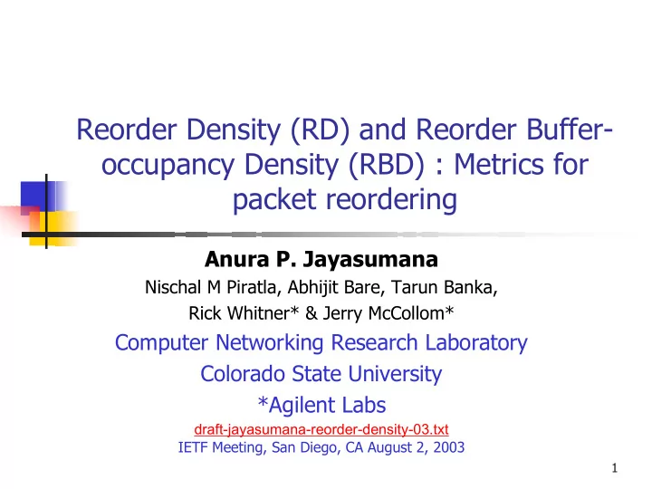
Reorder Density (RD) and Reorder Buffer- occupancy Density (RBD) : Metrics for packet reordering Anura P. Jayasumana Nischal M Piratla, Abhijit Bare, Tarun Banka, Rick Whitner* & Jerry McCollom* Computer Networking Research Laboratory Colorado State University *Agilent Labs draft-jayasumana-reorder-density-03.txt IETF Meeting, San Diego, CA August 2, 2003 1

Revision History � Reorder Buffer-occupancy Density (RBD) � The “Reorder Density” function defined in the previous draft is renamed RBD � New version of RBD is orthogonal to loss and duplication � First version of RBD useful from application point of view for recovery from reordering � Reorder Density (RD) – A comprehensive metric for reordering � Contains all information in ED (Early Density) and LD (Late Density) � Several useful properties including the ability to combine reorder information from subnets � Built in recovery features – burst losses, very early packets etc. 2

Concept of RBD Reorder Density Computation Module Incoming B T Sequence In-order Number Removal Occupancy If a packet with a sequence number higher than the currently � expected packet arrives, it is buffered. Packets are removed from the buffer, when they become in- � order or when the buffer is full. Occupancy of the buffer is recorded after each arrival is � processed. Size of the buffer (B T ) determines when a packet is considered � lost or useless. 3

Concept of RBD � Concern expressed at prior meeting: Dependency of metric on loss � New version: Modify buffer-occupancies to ignore losses � if a packet does not arrive even after the buffer is full (go-back BT), or � lag by BT delay detecting losses (stay-back BT). 4

Salient Features of RBD � New version: Orthogonal to loss and duplication � Earlier version: Useful for application from the point of recovery at the destination, e.g., estimation of buffer allocation requirements � Complexity: � Space complexity O(BT) � Computation complexity O(N) 5

RBD Measurements: With and Without Loss Detection 1.00 Without Loss Detection Without Loss Detection With Loss Detection With Loss Detection 0.98 0.9 0.96 0.94 Break from 0.05 to 0.94 RBD Break from 0.2 to 0.85 RBD 0.005 0.01 0.000 0.00 0 2 4 6 8 10 12 14 0 2 4 6 8 10 12 14 Buffer-occpuancy Buffer-occupancy From 202.54.x.x to 129.82.x.x From 210.212.x.x to 129.82.x.x 6

Packet Reordering A: 1,2,8,3,4,5,6,7,9,10,11,… B: 1,3,4,5,6,7,2,8,9,10,11,… C: 1,2,4,3,5,6,7,8,9,10,11,… 7

Definition and Concept of RD Packet Reordering: (m + d m ) m Arr Arriva val 1 2 4 5 3 7 6 Receive_index Receive_index 1 2 3 4 5 6 7 Displaceme Displac ment nt 0 0 -1 -1 -1 -1 2 -1 -1 1 (d (d m ) Reorder Event r(m, d m ): If the receive_index assigned to packet m is (m+d m ), with d m ≠ 0 then a reordered event r(m, d m ) has occurred Earliness/Lateness: A packet is late if d m > 0, and early if d m < 0 Packet Reordering: Packet reordering is completely represented by the union of reorder events, R = {r(m, d )|d ≠ 0} U m m m For the above sequence R = {(3, 2), (4, -1), (5, -1), (6, 1), (7, -1)} 8

Definition and Concept of RD Ex. 1: No losses/ duplicates Arr Arriva val 1 2 4 5 3 7 6 Receive_index Receive_index 1 2 3 4 5 6 7 Displac Displaceme ment nt 0 0 -1 -1 -1 -1 2 -1 -1 1 (d (d m ) Displacement (D) Displacement (D) -1 -1 0 1 2 Frequency FLE[ Frequency FLE[D] D] 3 2 1 1 Norm Normalized alized 3/7 3/7 2/7 2/7 1/7 1/7 1/7 1/7 Frequency RD[D] Frequency R [D] 9

Concept of RD Ex. 2: With packet duplication 1 is duplicated Arr Arriva val 1 2 4 5 3 1 6 Receive_index Receive_index 1 2 3 4 5 - 6 Displac Displaceme ment nt 0 0 -1 -1 -1 -1 2 - 0 Displacement (D) Displacement (D) -1 -1 0 1 2 Frequency FLE[ Frequency FLE[D] D] 2 3 0 1 Norm Normalized alized 2/6 2/6 3/6 3/6 0 1/6 1/6 Frequency RD[D] Frequency R [D] 10

Concept of RD Ex. 3: With packet loss, DT=2 5 is lost Arr Arriva val 1 3 4 2 6 7 8 Receive_index Receive_index 1 2 3 4 6 7 8 Displac Displaceme ment nt 0 -1 -1 -1 -1 2 0 0 0 Displacement (D) Displacement (D) -1 -1 0 1 2 Frequency FLE[ Frequency FLE[D] D] 2 4 0 1 Norm Normalized alized 2/7 2/7 4/7 4/7 0 1/7 1/7 Frequency RD[D] Frequency R [D] 11

RD Definition Let S[k] be a subset of R s.t S[k] = {r(m, d )|d = k} m m Then, RD [k] = |S[k]| / N ' for k ≠ 0 Where N ‘ is the total non-duplicate packets received and |S[k]| is cardinality of set S[k]. ∑ |S[k]|/N' RD[0] = 1 - k 0 ≠ 12

Methodology Assignment of receive_index values � Do not assign receive_index values for lost packets � Discard duplicate arrivals, i.e., no receive_index values � for such arrivals Result: Orthogonal to loss and duplication Detection of lost packets � Detection of duplicate packets � 13

Methodology - Detecting lost packets A packet is lost, if it is not within next DT arrivals, w.r.t � where it was in the ordered sequence Two detection methods: � Go-back DT: � � RD is computed in real-time � For previous DT arrivals, receive_index values are reassigned and RD is computed again, only if a packet is lost Stay-back DT: � � RD is computed with a lag DT arrivals � Next DT arrivals are checked for any lost packets before assigning the current receive_index value 14

Methodology – Detecting duplicates A packet is duplicate, if it is among early arrivals � Due to DT threshold on loss, the number of early � arrivals to be recorded is DT for the worst case 15

RD with Stay-back Procedure � Ex. 1 ( 1, 3, 4, 2, 6, 7, 8) with DT = 2 1, 3, 4, 2, 6, 7, 8) with DT = 2 1 3 4 window Arr Arriva val 1 3 4 Receive_index Receive_index 1 Displaceme Displac ment nt 0 16

RD with Stay-back Procedure � Ex. 1 ( 1, 3, 4, 2, 6, 7, 8) with DT = 2 1, 3, 4, 2, 6, 7, 8) with DT = 2 3 4 2 window 3 Early arrivals Arr Arriva val 1 3 4 2 Receive_index Receive_index 1 2 Displac Displaceme ment nt 0 -1 -1 17

RD with Stay-back Procedure � Ex. 1 ( 1, 3, 4, 2, 6, 7, 8) with DT = 2 1, 3, 4, 2, 6, 7, 8) with DT = 2 4 2 6 window 3 4 Early arrivals delete Arr Arriva val 1 3 4 2 6 Receive_index Receive_index 1 2 3 Displac Displaceme ment nt 0 -1 -1 -1 -1 18

RD with Stay-back Procedure � Ex. 1 ( 1, 3, 4, 2, 6, 7, 8) with DT = 2 1, 3, 4, 2, 6, 7, 8) with DT = 2 2 6 7 window 4 Early arrivals delete Arriva Arr val 1 3 4 2 6 7 Receive_index Receive_index 1 2 3 4 Displaceme Displac ment nt 0 -1 -1 -1 -1 2 19

RD with Stay-back Procedure � Ex. 1 ( 1, 3, 4, 2, 6, 7, 8) with DT = 2 1, 3, 4, 2, 6, 7, 8) with DT = 2 5 is lost 6 7 8 window Early arrivals Arriva Arr val 1 3 4 2 6 7 8 Receive_index Receive_index 1 2 3 4 6 7 8 Displaceme Displac ment nt 0 -1 -1 -1 -1 2 0 0 0 20

Salient Features of RD � As length of the sequence being evaluated increases, RD approaches the PDF of the packet displacement � Orthogonal to loss and duplication � Robustness – Receive_index self correcting in presence of losses, burst losses, sense of proportionality � Usefulness: Ex. Can be used for setting TCP parameter “dupthresh” dynamically � Complexity: � Space complexity O(DT) � Computation complexity O(N) � Broader applicability: Reorder Response 21

Reorder Response X Y [J] Subnet A Subnet A Reorder response of a network [J]: RD at the output of the subnet for a sequence of in-order packets A reorder response exists for a network in which the packet reordering � is not based on packet sequence number. The reorder response depends on the distribution of inter-packet gaps � and the network operating condition The reorder density Y at the output of the subnet for an out-of-order � input packet sequence with RD X is given by Y = X * J Ref: Reorder Density – A Metric for Packet Reordering, Piratla, Bare & � Jayasumana. See also http://www.cnrl.colostate.edu 22

RD and Reorder Response Net-X: Net-Y Net-X: Net-Y At steady conditions: D: 150ms D: 100ms D: 150ms D: 100ms SD: 7 ms SD: 4 ms SD: 7 ms SD: 4 ms A C B The reorder response J [ k ] of a network formed by cascading two subnets, with reorder responses 0.6 For N et-X (A to B) For N et-Y (B to C ) 0.4 J1 [ k ] and J2 [ k ] respectively, is 0.2 given by the convolution of J1 [ k ] 0.0 -6 -3 0 3 6 9 12 (a) RD and J2 [ k ] , i.e., 0.3 From A to C J [ k ] = J1 [ k ] * J2 [ k ]. U sing convolution theorem 0.2 0.1 0.0 -6 -3 0 3 6 9 12 Earliness/Lateness (b) 23

Resources � Our site http://www.cnrl.colostate.edu � Algorithms � Perl Scripts � Java Applets � Papers on Reordering � Information on Work in Progress 24

Future � Merge two drafts? � A separate ippm draft ? � An informational RFC � Further publications outside IETF 25