Regression and Difference of Two Proportions August 28, 2019 August - PowerPoint PPT Presentation
Regression and Difference of Two Proportions August 28, 2019 August 28, 2019 1 / 34 Regression Example The faithful dataset in R has two measurements taken for the Old Faithful Geyser in Yellowstone National Park: eruptions : the length of each
Regression and Difference of Two Proportions August 28, 2019 August 28, 2019 1 / 34
Regression Example The faithful dataset in R has two measurements taken for the Old Faithful Geyser in Yellowstone National Park: eruptions : the length of each eruption waiting : the time between eruptions Each is measured in minutes. Section 8.2 August 28, 2019 2 / 34
Regression Example We want to see if we can use the wait time to predict eruption duration. eruptions will be the response variable. waiting will be the predictor variable. Section 8.2 August 28, 2019 3 / 34
Regression Example Section 8.2 August 28, 2019 4 / 34
Regression Example Using R , the estimated regression line for eruptions = β 0 + β 1 waiting + ǫ is found to be y = − 1 . 8740 + 0 . 0756 x ˆ Section 8.2 August 28, 2019 5 / 34
Regression Example Section 8.2 August 28, 2019 6 / 34
Regression Example In this data, waiting times range from 43 minutes to 96 minutes. Let’s predict eruption time for a 50 minute wait. eruption time for a 10 minute wait. Section 8.2 August 28, 2019 7 / 34
Regression Example For waiting = x = 50, y = − 1 . 8740 + 0 . 0756 x ˆ = − 1 . 8740 + 0 . 0756 × 50 = 1 . 906 So for a wait time of 50 minutes, the predicted average eruption time is 1.906 minutes. Section 8.2 August 28, 2019 8 / 34
Regression Example For waiting = x = 10, y = − 1 . 8740 + 0 . 0756 x ˆ = − 1 . 8740 + 0 . 0756 × 10 = − 1 . 118 So for a wait time of 10 minutes, the predicted average eruption time is -1.118 minutes. Section 8.2 August 28, 2019 9 / 34
Regression Example But a predicted average eruption time of -1.118 minutes 1 doesn’t make sense. 2 is an extrapolation! We do not want to make this prediction. Section 8.2 August 28, 2019 10 / 34
Regression Example This is the residual plot for the geyser regression. Do you see any problems? Section 8.2 August 28, 2019 11 / 34
Regression Example This is a histogram of the residuals. Do they look normally distributed? Section 8.2 August 28, 2019 12 / 34
Regression Example Asking R for a summary of the regression model, we get the following: Let’s pick this apart piece by piece. Section 8.2 August 28, 2019 13 / 34
Regression Example The first line shows the command used in R to run this regression model. The Residuals item shows a quartile-based summary of our residuals. Section 8.2 August 28, 2019 14 / 34
Regression Example The F-statistic and p-value give information about the model overall. These are based on an F-distribution. The null hypothesis is that all of our model parameters are 0 (the model gives us no good info). Since p-value < 2 . 2 × 10 − 16 < α = 0 . 05, at least one of the parameters is nonzero (the model is useful). Section 8.2 August 28, 2019 15 / 34
Regression Example Multiple R-squared is our squared correlation coefficient R 2 . Ignore the adjusted R-squared and residual standard error for now. Section 8.2 August 28, 2019 16 / 34
Regression Example Finally, the Coefficients section gives us several pieces of information: 1 Estimate shows the estimated parameters for each value. 2 Std. Error gives the standard error for each parameter estimate. 3 The t values s are the test statistics for each parameter estiamte. 4 Finally, Pr(>|t|) are the p-values for each parameter estimate. Section 8.2 August 28, 2019 17 / 34
Regression Example The hypothesis test for each regression coefficient has hypotheses H 0 : β i = 0 H A : β i � = 0 where i = 0 for the intercept and i = 1 for the slope. Section 8.2 August 28, 2019 18 / 34
Regression Example 1 p − value < 2 × 10 − 16 for b 0 so we can conclude that the intercept is nonzero. 2 p − value < 2 × 10 − 16 for b 1 so we conclude that the intercept is also nonzero. 3 This means that the intercept and slope both provide useful information when predicting values of y = eruptions . Section 8.2 August 28, 2019 19 / 34
Difference of Two Proportions We will extend the methods for hypothesis tests for p to methods for p 1 − p 2 . This is the difference of proportions for two different groups or populations. The point estimate for p 1 − p 2 is ˆ p 1 − ˆ p 2 . We will develop a framework for use of the normal distribution and a new standard error formula. Section 6.2 August 28, 2019 20 / 34
Conditions for Normality p 1 − ˆ ˆ p 2 may be modeled using a normal distribution when The data are independent within and between groups. This should hold if the data from from a randomized experiment or from two independent random samples. Success-failure condition holds for both groups. n 1 p 1 ≥ 10 and n 1 (1 − p 1 ) ≥ 10 and n 2 p 2 ≥ 10 and n 2 (1 − p 2 ) ≥ 10 Section 6.2 August 28, 2019 21 / 34
Standard Error When the normality conditions hold, the standard error of ˆ p 1 − ˆ p 2 is � p 1 (1 − p 1 ) + p 2 (1 − p 2 ) SE = n 1 n 2 where p 1 and p 2 are the proportions and n 1 and n 2 are their respective sample sizes. Section 6.2 August 28, 2019 22 / 34
Confidence Intervals We can again use our generic confidence interval formula point estimate ± critical value × SE now as � p 1 (1 − p 1 ) + p 2 (1 − p 2 ) p 1 − ˆ ˆ p 2 ± z α/ 2 n 1 n 2 Section 6.2 August 28, 2019 23 / 34
Confidence Intervals The intervals are interpreted as before. E.g.,: One can be 95% confident that the true difference in proportions is between lower bound and upper bound. Section 6.2 August 28, 2019 24 / 34
Hypothesis Tests: Example A 30-year study was conducted with nearly 90,000 female participants. During a 5-year screening period, each woman was randomized to one of two groups: regular mammograms or regular non-mammogram breast cancer exams. No intervention was made during the following 25 years of the study, and we’ll consider death resulting from breast cancer over the full 30-year period. Section 6.2 August 28, 2019 25 / 34
Hypothesis Tests: Example Over the 30-year period, of the 44,925 women receiving mammograms, 500 died from breast cancer. of the 44,910 women receiving other cancer detection exams, 505 died from breast cancer. Create a contingency table for these data. Section 6.2 August 28, 2019 26 / 34
Hypothesis Tests: Example Set up the hypotheses for these data. Section 6.2 August 28, 2019 27 / 34
Special Case When H 0 : p 1 = p 2 , we use a special pooled proportion to check the success-failure condition: total number of cases = ˆ number of ”yes” p 1 n 1 + ˆ p 2 n 2 p pooled = ˆ n 1 + n 2 Note that this is usually the null hypothesis used in tests for two proportions. Section 6.2 August 28, 2019 28 / 34
Hypothesis Tests: Example Let’s calculate ˆ p pooled or our mammograms example. We will use this to check the success-failure condition. Section 6.2 August 28, 2019 29 / 34
Pooled Standard Error When H 0 : p 1 = p 2 , the standard error is calculated as � p pooled (1 − p pooled ) + p pooled (1 − p pooled ) SE pooled = n 1 n 2 Section 6.2 August 28, 2019 30 / 34
Hypothesis Tests: Example Let’s find the point estimate and standard error for our mammograms example. Section 6.2 August 28, 2019 31 / 34
Test Statistic As before, the test statistic is calculated as ts = z = point estimate − null value = (ˆ p 1 − ˆ p 2 ) − (null value) SE SE Section 6.2 August 28, 2019 32 / 34
Hypothesis Tests: Example For our mammograms example, the null value is 0, so ts = z = (ˆ p 1 − ˆ p 2 ) SE The critical value is z α/ 2 . At the 0.05 level of significance, z 0 . 025 = 1 . 96. Section 6.2 August 28, 2019 33 / 34
Hypothesis Tests: Example Since | z 0 . 025 | = 1 . 96 > | z | = | − 0 . 17 | = 0 . 17, we fail to reject the null hypothesis. there is insufficient evidence to suggest that mammograms are either helpful or harmful. Section 6.2 August 28, 2019 34 / 34
Recommend
More recommend
Explore More Topics
Stay informed with curated content and fresh updates.
