Recursive Lattice Search: Hierarchical Heavy Hitters Revisited - PowerPoint PPT Presentation
Recursive Lattice Search: Hierarchical Heavy Hitters Revisited Kenjiro Cho IIJ Research Laboratory IMC17 November 2, 2017 Hierarchical Heavy Hitters (HHHs) identifying significant clusters across multiple planes - exploiting underlying
Recursive Lattice Search: Hierarchical Heavy Hitters Revisited Kenjiro Cho IIJ Research Laboratory IMC’17 November 2, 2017
Hierarchical Heavy Hitters (HHHs) • identifying significant clusters across multiple planes - exploiting underlying hierarchical IP address structures - e.g., (src, dst) address pairs • (1.2.3.4, *) → one-to-many: e.g., scanning • (*, 5.6.7.8) → many-to-one: e.g., DDoS • (1.2.3.0/24, 4.5.6.0/28) → subnet-to-subnet - can be extended to higher dimensions (e.g., 5-tuple) • powerful tool for traffic monitoring/anomaly detection 2
Unidimensional HHH • an HHH: an aggregate with count c ≥ φ N - φ : threshold N : total input (e.g., packets or bytes) • HHHs can be uniquely identified by depth-first tree traversal - aggregating small nodes until it exceeds the threshold 0.0.0.0/0 0.0.0.0/0 10.1/16 192.168/16 10.1/16 192.168/16 192.168.3/24 192.168.3/24 10.1.1/24 10.1.2/24 10.1.1/24 10.1.2/24 3 10.1.1.4 10.1.2.5 10.1.1.4 10.1.2.5
Multi-dimensional HHH sum of prefix lengths 0,0 0 8,0 0,8 • each node has multiple parents 8 8,8 0,16 16,0 - many combinations for aggregation 16 8,16 24,0 0,24 16,8 - much harder than one-dimension 24 16,16 24,8 8,24 32,0 0,32 • search space for 2-dimensional IPv4 addrs 32 16,24 24,16 8,32 32,8 - 5×5=25 for bytewise aggregation 40 32,16 24,24 16,32 - 33×33=1089 for bitwise aggregation 48 src: 1.2.3.4 dst: 5.6.7.8 32,24 24,32 56 32,32 [1.2.3.4/32,5.6.0.0/16] [1.2.3.0/24,5.6.7.0/24] [1.2.0.0/16,1.2.3.4/32] 64 Lattice for IPv4 prefix length pair [1.2.3.4/32,5.6.7.0/24] [1.2.3.0/24,5.6.7.8/32] with 8-bit granularity [1.2.3.4/32,5.6.7.8/32] 4
Challenges • performance - bitwise aggregation is costly • operational relevance - ordering: e.g., [32, *] and [16, 16] - broad and redundant aggregates: (e.g., 128/4 and 128/2) • re-aggregation - useful for interactive analysis (for zoom-in/out) 5
Contributions into a tractable one, by revisiting the commonly accepted definition • new efficient HHH algorithm for bitwise aggregation - matches operational needs, supports re-aggregation • open-source tool and open datasets • more broadly, transforming the existing hard problem 6
Various HHH definitions • discounted HHH ⬅ we also employ this - exclude descendant HHHs’ counts for concise outputs c i ′ = ∑ j c j ′ where { j ∈ child(i) | c j ′ < φ N } • rollup rules: how to aggregate counts to parent - overlap rule: allows double-counting to detect all possible HHHs - split rule: preserves counts ⬅ we use a simple first-found split rule • aggregation ordering - sum of prefix lengths ⬅ we’ll revisit this ordering 7
Previous algorithms • elaborate structures - cross-producting, grid-of-trie, rectangle-search • theoretical analyses - streaming approximation algorithms w/ error bounds • all the existing methods are bottom-up • our algorithm: top-down, deterministic - no elaborate structure, no approximation, no parameter 8
HHH revisited • key idea: redefine child(i) to allow space partitioning - child(i) : from bin-tree to quadtree [16, 16] [16, 16] (1.2/16, 5.6/16) [16, 16] [24, 16] [16, 24] [24, 24] [24, 16] [16, 24] (1.2.0/24, 5.6/16) (1.2/16, 5.6.0/24) (1.2.1/24, 5.6/16) (1.2/16, 5.6.1/24) (1.2.3/24, 5.6/16) (1.2/16, 5.6.3/24) ... ... bottom-up aggregation top-down space partitioning 9
Z-order [Morton1966] dimensions • a space filling curve 0,0 - by bit-interleaving (l 0 , l 1 ) 8,0 0,8 8,8 0,16 16,0 8,16 24,0 16,8 0,24 • prefers the largest value across 24,8 8,24 16,16 32,0 0,32 16,24 24,16 8,32 32,8 24,24 32,16 16,32 • looks different from standard Z-curve 32,24 24,32 - [0..32] doesn’t have full 5-bit space 32,32 0,0 0,16 16,0 16,16 0,32 32,0 32,32 0,8 8,0 8,8 0,24 8,16 8,24 16,8 24,0 24,8 16,24 24,16 24,24 8,32 16,32 24,32 32,8 32,16 32,24 (I) upper (II) right (III) left (IV) lower (V) right (VI) left - makes /32 higher in the order sub-area sub-area sub-area sub-area bottom edge bottom edge 10
Recursive spatial partitioning • (VI) left-bottom edge • (V) right-bottom edge • (IV) lower quadrant • (III) left quadrant • (II) right quadrant • (I) upper quadrant 0,0 • visit regions from (VI) to (I) recursively 8,0 0,8 - 2 bottom edges 8,8 0,16 16,0 (I) 8,16 24,0 0,24 16,8 24,8 16,16 8,24 32,0 0,32 - 4 quadrants (III) (II) 16,24 24,16 32,8 8,32 32,16 16,32 24,24 (VI) (VI) (V) (V) (IV) 32,24 24,32 32,32 11
Recursive Lattice Search (RLS) • idea: recursively subdivide aggregates by Z-order • pros - recurse only for flows ≥ thresh - sub-division needs only parent’s sub-flows - /32 becomes higher in the order • cons - bias for the first dimension 12
RLS Illustrated 0,0 10 inputs, HHH ≥ 2 16,0 0,16 16,16 32,0 0,32 32,16 16,32 32,32 13
RLS Illustrated 0,0 10 inputs, HHH ≥ 2 16,0 0,16 16,16 32,0 0,32 32,16 16,32 32,32 13
RLS Illustrated 0,0 10 inputs, HHH ≥ 2 16,0 0,16 16,16 32,0 0,32 32,16 16,32 32,32 13
RLS Illustrated 0,0 10 inputs, HHH ≥ 2 16,0 0,16 16,16 32,0 0,32 32,16 16,32 32,32 13
RLS Illustrated 0,0 10 inputs, HHH ≥ 2 16,0 0,16 16,16 32,0 0,32 32,16 16,32 32,32 13
RLS Illustrated 0,0 10 inputs, HHH ≥ 2 16,0 0,16 16,16 32,0 0,32 32,16 16,32 32,32 13
RLS Illustrated 0,0 10 inputs, HHH ≥ 2 16,0 0,16 16,16 32,0 0,32 32,16 16,32 32,32 13
RLS Illustrated 0,0 10 inputs, HHH ≥ 2 16,0 0,16 16,16 32,0 0,32 32,16 16,32 32,32 13
RLS Illustrated 0,0 10 inputs, HHH ≥ 2 16,0 0,16 16,16 32,0 0,32 32,16 16,32 32,32 13
RLS Illustrated 0,0 10 inputs, HHH ≥ 2 16,0 0,16 16,16 32,0 0,32 32,16 16,32 32,32 13
RLS Illustrated 0,0 10 inputs, HHH ≥ 2 16,0 0,16 16,16 32,0 0,32 32,16 16,32 32,32 13
RLS Illustrated 0,0 10 inputs, HHH ≥ 2 16,0 0,16 16,16 32,0 0,32 32,16 16,32 32,32 13
RLS Illustrated 0,0 10 inputs, HHH ≥ 2 16,0 0,16 16,16 32,0 0,32 32,16 16,32 32,32 13
RLS Illustrated 0,0 10 inputs, HHH ≥ 2 16,0 0,16 16,16 32,0 0,32 32,16 16,32 32,32 13
RLS Illustrated 0,0 10 inputs, HHH ≥ 2 16,0 0,16 16,16 32,0 0,32 32,16 16,32 32,32 13
RLS Illustrated 0,0 10 inputs, HHH ≥ 2 16,0 0,16 16,16 32,0 0,32 32,16 16,32 32,32 13
RLS Illustrated 0,0 10 inputs, HHH ≥ 2 16,0 0,16 16,16 32,0 0,32 32,16 16,32 32,32 13
RLS Illustrated 0,0 10 inputs, HHH ≥ 2 16,0 0,16 16,16 32,0 0,32 32,16 16,32 32,32 13
RLS Illustrated 0,0 10 inputs, HHH ≥ 2 16,0 0,16 16,16 32,0 0,32 32,16 16,32 32,32 13
RLS Illustrated 0,0 10 inputs, HHH ≥ 2 16,0 0,16 16,16 32,0 0,32 32,16 16,32 32,32 13
RLS Illustrated 0,0 10 inputs, HHH ≥ 2 16,0 0,16 16,16 32,0 0,32 32,16 16,32 32,32 13
RLS Illustrated 0,0 10 inputs, HHH ≥ 2 16,0 0,16 16,16 32,0 0,32 32,16 16,32 32,32 13
RLS Illustrated 0,0 10 inputs, HHH ≥ 2 16,0 0,16 16,16 32,0 0,32 32,16 16,32 32,32 13
RLS Illustrated 0,0 10 inputs, HHH ≥ 2 4 HHHs extracted 16,0 0,16 16,16 32,0 0,32 32,16 16,32 32,32 13
Evaluation (in the paper) • differences due to different definitions • but requires more memory (as a non-streaming algo) • ordering bias: (src, dst) vs (dst, src) ➡ negligible • comparison with Space-Saving: to illustrate differences - outputs ➡ much more compact - speed ➡ 100 times faster for bitwise aggregation 14
meet operational needs Implementations: RLS in agurim • agurim: open-source tool • 2-level HHH - main-attribute (src-dst adds), sub-attritbute (ports) • protocol specific heuristics - change depth of recursions by protocol knowledge to • online processing by exploiting multi-core CPU 15
agurim Web UI http://mawi.wide.ad.jp/~agurim/ 16
Summary • Recursive Lattice Search algorithm for HHH - revisit the definition of HHH, apply Z-ordering - propose an efficient HHH algorithm • open-source tool and open datasets from 2013 http://mawi.wide.ad.jp/~agurim/about.html 17
evaluation in detail • simulation: code from SpaceSaving [Mitzenmacher2012] - quick hack to port agurim’s RLS - input: a mawi packet trace from 2016-10-20 • order sensitivity: (src,dst) vs. (dst,src) - very similar outputs: not sensitive to the order • comparing with SS (streaming algorithm, overlap rollup) - different definitions: just to illustrate major differences - outputs: comparable, except nodes in upper lattice - performance: 100x faster for bit-wise aggregation! 18
Recommend
More recommend
Explore More Topics
Stay informed with curated content and fresh updates.


