Recap Hashing-based sketch techniques summarize large data sets - - PowerPoint PPT Presentation

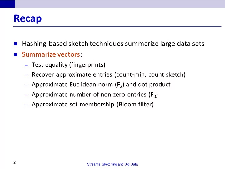
Recap

 Hashing-based sketch techniques summarize large data sets  Summarize vectors:

– Test equality (fingerprints) – Recover approximate entries (count-min, count sketch) – Approximate Euclidean norm (F2) and dot product – Approximate number of non-zero entries (F0) – Approximate set membership (Bloom filter)

Streams, Sketching and Big Data

2

Advanced Topics

 Lp Sampling

– L0 sampling and graph sketching – L2 sampling and frequency moment estimation

 Matrix computations

– Sketches for matrix multiplication – Compressed matrix multiplication

 Hashing to check computation

– Matrix product checking – Vector product checking

 Lower bounds for streaming and sketching

– Basic hard problems (Index, Disjointness) – Hardness via reductions

Streams, Sketching and Big Data

3

Sampling from Sketches

 Given inputs with positive and negative weights  Want to sample based on the overall frequency distribution

– Sample from support set of n possible items – Sample proportional to (absolute) weights – Sample proportional to some function of weights

 How to do this sampling effectively?  Recent approach: Lp sampling

Streams, Sketching and Big Data

4

Lp Sampling

 Lp sampling: use sketches to sample i w/prob (1±e) fi

p/ǁfǁp p

 “Efficient” solutions developed of size O(e-2 log2 n)

– [Monemizadeh, Woodruff 10] [Jowhari, Saglam, Tardos 11]

 L0 sampling enables novel “graph sketching” techniques

– Sketches for connectivity, sparsifiers [Ahn, Guha, McGregor 12]

 L2 sampling allows optimal estimation of frequency moments

Streams, Sketching and Big Data

5

L0 Sampling

 L0 sampling: sample with prob (1±e) fi

0/F0

– i.e., sample (near) uniformly from items with non-zero frequency

 General approach: [Frahling, Indyk, Sohler 05, C., Muthu, Rozenbaum 05]

– Sub-sample all items (present or not) with probability p – Generate a sub-sampled vector of frequencies fp – Feed fp to a k-sparse recovery data structure

 Allows reconstruction of fp if F0 < k

– If fp is k-sparse, sample from reconstructed vector – Repeat in parallel for exponentially shrinking values of p

Streams, Sketching and Big Data

6

Sampling Process

 Exponential set of probabilities, p=1, ½, ¼, 1/8, 1/16… 1/U

– Let N = F0 = |{ i : fi  0}| – Want there to be a level where k-sparse recovery will succeed – At level p, expected number of items selected S is Np – Pick level p so that k/3 < Np  2k/3

 Chernoff bound: with probability exponential in k, 1  S  k

– Pick k = O(log 1/) to get 1- probability

Streams, Sketching and Big Data

p=1 p=1/U k-sparse recovery

7

k-Sparse Recovery

 Given vector x with at most k non-zeros, recover x via sketching

– A core problem in compressed sensing/compressive sampling

 First approach: Use Count-Min sketch of x

– Probe all U items, find those with non-zero estimated frequency – Slow recovery: takes O(U) time

 Faster approach: also keep sum of item identifiers in each cell

– Sum/count will reveal item id – Avoid false positives: keep fingerprint of items in each cell

 Can keep a sketch of size O(k log U) to recover up to k items

Streams, Sketching and Big Data

Sum, i : h(i)=j i Count, i : h(i)=j xi Fingerprint, i : h(i)=j xi ri

8

Uniformity

 Also need to argue sample is uniform

– Failure to recover could bias the process

 Pr[ i would be picked if k=n] = 1/F0 by symmetry  Pr[ i is picked ] = Pr[ i would be picked if k=n  S k]

 (1-)/F0

 So (1-)/N  Pr[i is picked]  1/N  Sufficiently uniform (pick  = e)

Streams, Sketching and Big Data

9

Application: Graph Sketching

 Given L0 sampler, use to sketch (undirected) graph properties  Connectivity: want to test if there is a path between all pairs  Basic alg: repeatedly contract edges between components  Use L0 sampling to provide edges on vector of adjacencies  Problem: as components grow, sampling most likely to

produce internal links

Streams, Sketching and Big Data

10

Graph Sketching

 Idea: use clever encoding of edges [Ahn, Guha, McGregor 12]  Encode edge (i,j) as ((i,j),+1) for node i<j, as ((i,j),-1) for node j>i  When node i and node j get merged, sum their L0 sketches

– Contribution of edge (i,j) exactly cancels out

 Only non-internal edges remain in the L0 sketches  Use independent sketches for each iteration of the algorithm

– Only need O(log n) rounds with high probability

 Result: O(poly-log n) space per node for connectivity

Streams, Sketching and Big Data

i j + =

11

Other Graph Results via sketching

 K-connectivity via connectivity

– Use connectivity result to find and remove a spanning forest – Repeat k times to generate k spanning forests F1, F2, … Fk – Theorem: G is k-connected if i=1k Fi is k-connected

 Bipartiteness via connectivity:

– Compute c = number of connected components in G – Generate G’ over V  V’ so (u,v)  E  (u, v’)  E’, (u’, v)  E’ – If G is bipartite, G’ has 2c components, else it has <2c components

 (Weight of the) Minimum spanning tree:

– Round edge weights to powers of (1+e) – Define ni = number of components on edges lighter than (1+e)i – Fact: weight of MST on rounded weights is i e(1+e)ini

Streams, Sketching and Big Data

12

Application: Fk via L2 Sampling

 Recall, Fk = i fi

k

 Suppose L2 sampling samples fi with probability fi

2/F2

– And also estimates sampled fi with relative error e

 Estimator: X = F2 fi

k-2 (with estimates of F2, fi)

– Expectation: E[X] = F2 i fik-2  fi2 / F2 = Fk – Variance: Var[X]  E[X2] = i fi2/F2 (F2 fik-2)2 = F2 F2k-2

Streams, Sketching and Big Data

13

Rewriting the Variance

 Want to express variance F2 F2k-2 in terms of Fk and domain size n  Hölder’s inequality: x, y  ǁxǁp ǁyǁq for 1  p, q with 1/p+1/q=1

– Generalizes Cauchy-Shwarz inequality, where p=q=2.

 So pick p=k/(k-2) and q = k/2 for k > 2. Then

 1n, (fi)2  ǁ1nǁk/(k-2) ǁ(fi)2ǁk/2 F2 n(k-2)/k Fk

2/k

(1)

 Also, since ǁxǁp+a  ǁxǁp for any p 1, a > 0

– Thus ǁxǁ2k-2  ǁxǁk for k  2 – So F2k-2 = ǁfǁ2k-22k-2  ǁfǁk2k-2 = Fk2-2/k

(2)

 Multiply (1) * (2) : F2 F2k-2  n1-2/k Fk

2

– So variance is bounded by n1-2/k Fk2

Streams, Sketching and Big Data

14

Fk Estimation

 For k  3, we can estimate Fk via L2 sampling:

– Variance of our estimate is O(Fk2 n1-2/k) – Take mean of n1-2/ke-2 repetitions to reduce variance – Apply Chebyshev inequality: constant prob of good estimate – Chernoff bounds: O(log 1/) repetitions reduces prob to 

 How to instantiate this?

– Design method for approximate L2 sampling via sketches – Show that this gives relative error approximation of fi – Use approximate value of F2 from sketch – Complicates the analysis, but bound stays similar

Streams, Sketching and Big Data

15

L2 Sampling Outline

 For each i, draw ui uniformly in the range 0…1

– From vector of frequencies f, derive g so gi = fi/√ui – Sketch gi vector

 Sample: return (i, fi) if there is unique i with gi

2 > t=F2/e threshold

– Pr[ gi2 > t   j  i : gj2 < t]= Pr[gi2 > t] ji Pr[gj2 < t]

= Pr[ui < efi2/F2] ji Pr[uj > efj2/F2] = (efi2/F2 ) ji (1 - efj2/F2) ≈ efi2/F2

 Probability of returning anything is not so big: i e fi

2/F2 = e

– Repeat O(1/e log 1/) times to improve chance of sampling

Streams, Sketching and Big Data

16

L2 sampling continued

 Given (estimated) gi s.t. gi

2  F2/e, estimate fi = ui gi

 Sketch size O(e-1 log n) means estimate of fi

2 has error (efi 2 + ui 2)

– With high prob, no ui < 1/poly(n), and so F2(g) = O(F2(f) log n) – Since estimated fi2/ui2  F2/e, ui2  efi2/F2

 Estimating fi

2 with error efi 2 sufficient for estimating Fk

 Many details omitted

–

See Precision Sampling paper [Andoni Krauthgamer Onak 11]

Streams, Sketching and Big Data

17

Advanced Topics

 Lp Sampling

– L0 sampling and graph sketching – L2 sampling and frequency moment estimation

 Matrix computations

– Sketches for matrix multiplication – Compressed matrix multiplication

 Hashing to check computation

– Matrix product checking – Vector product checking

 Lower bounds for streaming and sketching

– Basic hard problems (Index, Disjointness) – Hardness via reductions

Streams, Sketching and Big Data

18

Matrix Sketching

 Given matrices A, B, want to approximate matrix product AB  Compute normed error of approximation C: ǁAB – Cǁ  Give results for the Frobenius (entrywise) norm ǁǁF

– ǁCǁF = (i,j Ci,j2)½ – Results rely on sketches, so this norm is most natural

Streams, Sketching and Big Data

19

Direct Application of Sketches

 Build sketch of each row of A, each column of B  Estimate Ci,j by estimating inner product of Ai with Bj  Absolute error in estimate is e ǁAiǁ2 ǁBjǁ2 (whp)  Sum over all entries in matrix, squared error is

e2 i,j ǁAiǁ2

2 ǁBjǁ2 2 = e2 (i ǁAiǁ2 2)(j ǁBjǁ2 2)

= e2 (ǁAǁF

2)(ǁBǁF 2)

 Hence, Frobenius norm of error is eǁAǁFǁBǁF  Problem: need the bound to hold for all sketches simultaneously

– Requires polynomially small failure probability – Increases sketch size by logarithmic factors

Streams, Sketching and Big Data

20

Improved Matrix Multiplication Analysis

 Simple analysis is too pessimistic [Clarkson Woodruff 09]

– It bounds probability of failure of each sketch independently

 A better approach is to directly analyze variance of error

– Immediately, each estimate of (AB) has variance e2ǁAǁF2ǁBǁF2 – Just need to apply Chebyshev inequality to this… almost

 Problem: how to amplify probability of correctness?

– ‘Median’ trick doesn’t work: what is median of set of matrices? – Find an estimate which is close to most others

 Estimate ǁAǁF2ǁBǁF2 := d using sketches  Find an estimate that’s closer than d/2 to more than ½ the rest  We find an estimate with this property with probability 1-

Streams, Sketching and Big Data

21

Compressed Matrix Multiplication

 What if we are just interested in the large entries of AB?

– Or, the ability to estimate any entry of (AB)

 If we had a sketch of (AB), could find these approximately  Compressed Matrix Multiplication [Pagh 12]:

– Can we compute sketch(AB) from sketch(A) and sketch(B)? – To do this, need to dive into structure of the Count (AMS) sketch

Streams, Sketching and Big Data

22

Compressed Matrix Multiplication

 Entry (AB)ij gets mapped by a pairwise hash function to a cell q  Idea: choose a carefully structured hash function

– h(i,j) = h1(i) + h2(j) (mod p) is pairwise, if h1 and h2 are parwise

 Take convolution of sketch(Ak) [with h1] and sketch(Bk ) [with h2]

– Cell q contains  Aik Bkj g(i) g(j) where h(i,j) = q – Repeat for all k and sum to get sketch(AB)

Streams, Sketching and Big Data

c*g1(j) c*g2(j) c*g3(j) c*g4(j)

h1(j) hd(j) i,j,c

23

Compressed Matrix Multiplication: Analysis

 Computing the convolution takes time O(w log w)

– Via Fast Fourier Transform

 Each sketch convolution builds sketch of k’th outer product

– Total time cost: O(n(n + w log w)) – Compared to superquadratic cost of exact matrix product – Estimate of (AB)ij has error ǁABǁF2/w

 Several insights needed to build the method:

– Express matrix product as summation of outer products – Convolution of sketches gives a sketch of outer product – FFT speeds up from O(w2) to O(w log w)

Streams, Sketching and Big Data

24

Advanced Linear Algebra

 Recent work more directly approximates matrix multiplication:

– use more powerful hash functions in sketching – obtain a single accurate estimate with high probability

 Linear regression given matrix A and vector b:

find x  Rd to (approximately) solve minx ǁAx – bǁ

– Approach: solve the minimization in “sketch space” – Require a summary of size O(d2/e log 1/)

Streams, Sketching and Big Data

25

Advanced Topics

 Lp Sampling

– L0 sampling and graph sketching – L2 sampling and frequency moment estimation

 Matrix computations

– Sketches for matrix multiplication – Compressed matrix multiplication

 Hashing to check computation

– Matrix product checking – Vector product checking

 Lower bounds for streaming and sketching

– Basic hard problems (Index, Disjointness) – Hardness via reductions

Streams, Sketching and Big Data

26

Streams, Sketching and Big Data

Outsourced Computation

 Current trend to ‘outsource’ computation

– Cloud computing: Amazon EC2, Microsoft Azure… – Hardware support: multicore systems, graphics cards

 We provide data to a third party, they return an answer  How can we be sure that the computation is correct?

– Duplicate the whole computation ourselves? – Find some ad hoc sanity checks on the answer?

 Hashing to the rescue: use hashing to prove the correctness

– Previously, use hashing to test correctness of data (fingerprints) – Now, use hashing to test correctness of computation – Protocols must be very low cost for the data owner (streaming) – Amount of information transmitted should not be too large

27

Example: Freivald’s Algorithm

 Goal: Check AB = C for n x n matrices A, B, C

– Naïve algorithm: compute AB, check = C – O(n2.37…) time

 Freivald’s: check ABrT = CrTfor random vector r

– A classic example of randomized algorithms, takes O(n2) time

 Variant: define r = [1, r, r2…rn] and s = [1, s, s2…sn] for random r, s  Check s(AB)rT = sCrT [ mod p ]

 Define hash function hr,s(X) = sXrT mod p = ij xij si rj mod p  Pr[h(AB) = h(C)] = Probability that a polynomial in r, s of total

degree 2n evaluates to 0 for randomly chosen variables = 2n/p

 p only has to be polynomial in n, so logarithmic number of bits

 Streaming friendly: compute (sA), (BrT) and (sCrT) incrementally

Streams, Sketching and Big Data

28

Streams, Sketching and Big Data

Streaming Proofs

 Objective: prove integrity of the computed solution

– Not concerned with security: third party sees unencrypted data

 Prover provides “proof” of the correct answer

– Ensure that “verifier” has very low probability of being fooled – Related to communication complexity Arthur-Merlin model, and

Arithmetization, with additional streaming constraints

Data Stream

P V

“Proof”

29

Streams, Sketching and Big Data

Inner Product Computation

 Given vectors a, b, defined in the stream, want to compute ab  Inner product appears in many problems

– Core computation in data streams – Requires (N) space to compute in traditional models

 Results: for h,v s.t. (hv) > N, there exists a protocol with proof

size O(h log m), and space O(v log m) to compute inner product

– Lower bounds: hv = (N) necessary for exact computation

30

Streams, Sketching and Big Data

Inner Product Protocol

 Map [N] to h  v array  Interpolate entries in array as polynomials a(x,y), b(x,y)  Verifier picks random r, evaluates a(r, j) and b(r,j) for j  [v]  Prover sends s(x) = j[v] a(x, j)b(x,j)(degree h)

– Verifier checks s(r) = j[v] a(r,j)b(r,j) – Output ab = i [h] s(i) if test passed

 Probability of failure small if evaluated

• ver large enough field

– A “Low Degree Extension” / arithmetization technique – Can view a(x,y), b(x,y) as (linear) hash functions of the data

3 7 1 2 0 8 5 9 1 1 1 0 3 7 1 2 0 8 5 9 1 1 1 0

31

Streams, Sketching and Big Data

Streaming Hash Functions

 Must evaluate a(r,j) incrementally as a() is defined by stream  Structure of polynomial means updates to (w,z) cause

a(r,j)  a(r,j) + pw,z(r,j) where pw,z(x,y) = i [h]\{w} (x-i)(w-i)-1j [v]\{z} (y-j)(z-j)-1

– p is a Lagrange polynomial corresponding to an impulse at (w,z)

 Can be computed quickly, using appropriate precomputed

look-up tables

 Evaluation is linear: can be computed over distributed data

32

Consequences

 Verifier can keep space O(√n), process proof of size O(√n) to

verify inner product of two vectors

 Many consequences of inner-product verification

– Easily check Euclidean norm of vector described in stream – Verify solutions to linear programs (evaluate primal and dual) – Graph computations, e.g. check connected components – Count triangles (expressed as polynomial over derived stream) – Flow computations (shortest paths, max flow) via IP formulation

Streams, Sketching and Big Data

33

Further Directions in Verification

 Multi-round protocols can reduce the costs exponentially

– Evaluate the low-degree extension of the data at one location – Functions as a hash function for computation

 “Interactive Proofs for Muggles” [Goldwasser et al 08]

– A general purpose approach to verifying computation as circuits – Implemented and evaluated by Thaler [Thaler 13]

 Much ongoing around verification

– Distributed/parallel versions of these protocols – Lower bounds for multi-round versions of the protocols – Engineering practical implementations

Streams, Sketching and Big Data

34

Advanced Topics

 Lp Sampling

– L0 sampling and graph sketching – L2 sampling and frequency moment estimation

 Matrix computations

– Sketches for matrix multiplication – Compressed matrix multiplication

 Hashing to check computation

– Matrix product checking – Vector product checking

 Lower bounds for streaming and sketching

– Basic hard problems (Index, Disjointness) – Hardness via reductions

Streams, Sketching and Big Data

35

Streams, Sketching and Big Data

Computation As Communication

 Imagine Alice processing a prefix of the input  Then takes the whole working memory, and sends to Bob  Bob continues processing the remainder of the input

1 0 1 1 1 0 1 0 1 …

Alice Bob

36

Streams, Sketching and Big Data

Computation As Communication

 Suppose Alice’s part of the input corresponds to string x, and

Bob’s part corresponds to string y...

 ...and computing the function corresponds to computing

f(x,y)...

 ...then if f(x,y) has communication complexity (CC) (g(n)),

then the computation has a space lower bound of (g(n))

 Proof by contradiction:

If there was an algorithm with better space usage, we could run it on x, then send the memory contents as a message, and hence solve the communication problem

37

Streams, Sketching and Big Data

Deterministic Equality Testing

 Alice has string x, Bob has string y, want to test if x=y  Consider a deterministic (one-round, one-way) protocol that

sends a message of length m < n

 There are 2m possible messages, so some strings must

generate the same message: this would cause error

 So a deterministic message (sketch) must be (n) bits

– In contrast, we saw a randomized sketch of size O(log n)

1 0 1 1 1 0 1 0 1 … 1 0 1 1 0 0 1 0 1 …

38

Streams, Sketching and Big Data

Four Hard Communication Problems

 INDEX: Alice’s x is binary string of length n, Bob’s y is index in [n]

Goal: output x[y] Result: one-way randomized CC of INDEX is (n) bits

 AUGINDEX: as INDEX, but Bob also receives x[y+1]…x[n]

Result: one-way randomized CC of AUGINDEX is (n) bits

 DISJ: Alice’s x and Bob’s y are both length n binary strings

Goal: Output 1 if i: x[i]=y[i]=1, else 0 Result: multi-round randomized CC of DISJ (disjointness) is (n) bits

 Gap-Hamming: Alice’s x and Bob’s y are both length n binary strings

Promise: Ham(x,y) is either  N/2 - √N or  N/2 + √N Goal: determine which case holds Result: multi-round randomized CC of Gap-Hamming is (n) bits

39

Streams, Sketching and Big Data

Simple Reduction to Disjointness

 F: output the highest frequency in the input  Input: the two strings x and y from disjointness instance  Reduction: if x[i]=1, then put i in input; then same for y

– A streaming reduction (compare to polynomial-time reductions)

 Analysis: if F=2, then intersection; if F1, then disjoint.  Conclusion: Giving exact answer to F requires (N)bits

– Even approximating up to 50% relative error is hard – Even with randomization: DISJ bound allows randomness

x: 1 0 1 1 0 1 y: 0 0 0 1 1 0 1, 3, 4, 6 4, 5

40

Streams, Sketching and Big Data

Simple Reduction to Index

 F0: output the number of items in the stream  Input: the strings x and index y from INDEX  Reduction: if x[i]=1, put i in input; then put y in input  Analysis: if (1-e)F’0(xy)>(1+e)F’0(x)then x[y]=1, else it is 0  Conclusion: Approximating F0 for e<1/N requires (N)bits

– Implies that space to approximate must be (1/e) – Bound allows randomization

x: 1 0 1 1 0 1 y: 5 1, 3, 4, 6 5

41

Reduction to AUGINDEX [Clarkson Woodruff 09]

 Matrix-Multiplication: approximate ATB with error e2ǁAǁF ǁBǁF

– For r  c matrices. A encodes string x, B encodes index y

 Bob uses suffix of x in y to remove heavy entries from A

ǁBǁF= 1 ǁAǁF = cr/log (cn) *(1 + 4 + … 22k)  4cr22k/3log (cn)

 Choose r = log(cn)/8e

2 so permitted error is c 22k / 6e2

– Each error in sign in estimate of (ATB) contributes 22k error – Can tolerate error in at most 1/6 fraction of entries

 Matrix multiplication requires space (rc) = (c/e2 log (cn))

Streams, Sketching and Big Data

+1 -1 -2 -2 … 2k 2k … 0 0 0 0 0

• 1 -1 -2 +2 … 2k 2k … 0 0 0 0 0

+1 +1 +2 -2 … 2k 2k … 0 0 0 0 0

• 1 -1 +2 +2 … 2k 2k … 0 0 0 0 0

[ ][

0 0 … 0 0 … 0 0 … 0 0 … 0 0 … 0 0 … 1 0 … 0 0 … 0 0 … 0 0 …]

c r/log(cn) ATB “reads off” j’th column of AT

42

Streams, Sketching and Big Data

Lower Bound for Entropy

Gap-Hamming instance—Alice: x  {0,1}N, Bob: y  {0,1}N Entropy estimation algorithm A

 Alice runs A on enc(x) = (1,x1), (2,x2), …, (N,xN)  Alice sends over memory contents to Bob  Bob continues A on enc(y) = (1,y1), (2,y2), …, (N,yN)

1 1 1 (6,0) (5,1) (4,0) (3,0) (2,1) (1,1) Bob (6,1) (5,1) (4,0) (3,0) (2,1) (1,0) 1 1 1 Alice

43

Streams, Sketching and Big Data

Lower Bound for Entropy

 Observe: there are

– 2Ham(x,y) tokens with frequency 1 each – N-Ham(x,y) tokens with frequency 2 each

 So (after algebra), H(S) = log N + Ham(x,y)/N = log N + ½  1/√N  If we separate two cases, size of Alice’s memory contents = (N)

Set e = 1/(√(N) log N) to show bound of (e/log 1/e)-2)

1 1 1 (6,0) (5,1) (4,0) (3,0) (2,1) (1,1) Bob (6,1) (5,1) (4,0) (3,0) (2,1) (1,0) 1 1 1 Alice

44

Streams, Sketching and Big Data

Lower Bound for F0

 Same encoding works for F0 (Distinct Elements)

– 2Ham(x,y) tokens with frequency 1 each – N-Ham(x,y) tokens with frequency 2 each

 F0(S) = N + Ham(x,y)  Either Ham(x,y)>N/2 + N or Ham(x,y)<N/2 - N

– If we could approximate F0 with e < 1/N, could separate – But space bound = (N) = (e-2) bits

 Dependence on e for F0 is tight  Similar arguments show (e-2) bounds for Fk

– Proof assumes k (and hence 2k) are constants

45

Summary of Tools

 Vector equality: fingerprints  Approximate item frequencies:

– Count-min (L1 guarantee), Count sketch (L2 guarantee)

 Euclidean norm, inner product: AMS sketch, JL sketches  Count-distinct: k-Minimum values, Hyperloglog  Compact set-representation: Bloom filters  L0 sampling:hashing and sparse recovery  L2 sampling: via count-sketch  Graph sketching: L0 samples of neighborhood  Frequency moments: via L2 sampling  Matrix sketches: adapt AMS sketches, compressed matrix multiplication

Streams, Sketching and Big Data

46

Summary of Lower Bounds

 Can’t deterministically test equality  Can’t retrieve arbitrary bits from a vector of n bits: INDEX

– Even if some unhelpful suffix of the vector is given: AUGINDEX

 Can’t determine whether two n bit vectors intersect: DISJ  Can’t distinguish small differences in Hamming distance:

GAP-HAMMING

 These in turn provide lower bounds on the cost of

– Finding the maximum frequency – Approximating the number of distinct items – Approximating matrix multiplication

Streams, Sketching and Big Data

47

Current Directions in Streaming and Sketching

 Sparse representations of high dimensional objects

– Compressed sensing, sparse fast fourier transform

 Numerical linear algebra for (large) matrices

– k-rank approximation, linear regression, PCA, SVD, eigenvalues

 Computations on large graphs

– Sparsification, clustering, matching

 Geometric (big) data

– Coresets, facility location, optimization, machine learning

 Use of summaries in distributed computation

– MapReduce, Continuous Distributed models

Streams, Sketching and Big Data

48