Reasoning with Bayes Bayes Networks Networks Reasoning with - PowerPoint PPT Presentation
Reasoning with Bayes Bayes Networks Networks Reasoning with Course: CS40022 Course: CS40022 Instructor: Dr. Pallab Dasgupta Pallab Dasgupta Instructor: Dr. Department of Computer Science & Engineering Department of Computer Science
Reasoning with Bayes Bayes Networks Networks Reasoning with Course: CS40022 Course: CS40022 Instructor: Dr. Pallab Dasgupta Pallab Dasgupta Instructor: Dr. Department of Computer Science & Engineering Department of Computer Science & Engineering Indian Institute of Technology Kharagpur Kharagpur Indian Institute of Technology
Belief Network Example Belief Network Example P(B) P(E) P(B) P(E) Burglary Earthquake 0.001 0.001 0.002 0.002 B E P(A) B E P(A) T T T T 0.95 0.95 Alarm T F 0.95 T F 0.95 F T 0.29 F T 0.29 F F 0.001 F F 0.001 A P(J) A P(J) T 0.90 A P(M) T 0.90 A P(M) JohnCalls MaryCalls F 0.05 T 0.70 F 0.05 T 0.70 F 0.01 F 0.01 CSE, IIT Kharagpur Kharagpur CSE, IIT
Answering queries Answering queries � We consider cases where the belief network We consider cases where the belief network � is a poly- -tree tree is a poly � There is at most one undirected path There is at most one undirected path � between any two nodes between any two nodes CSE, IIT Kharagpur Kharagpur CSE, IIT
Answering queries Answering queries + E X U 1 U m X − E X Z nj Z 1j Y 1 Y n CSE, IIT Kharagpur Kharagpur CSE, IIT
Answering queries Answering queries • U = U 1 … U m are parents of node X • Y = Y 1 … Y n are children of node X • X is the query variable • E is a set of evidence variables • The aim is to compute P(X | E) CSE, IIT Kharagpur Kharagpur CSE, IIT
Definitions Definitions + is the causal support for X � E E X is the causal support for X X+ � � The evidence variables “ The evidence variables “above above” X that are ” X that are � connected to X through its parents connected to X through its parents – is the evidential support for X � E E X is the evidential support for X X– � � The evidence variables “ The evidence variables “below below” X that are ” X that are � connected to X through its children connected to X through its children � E E Ui refers to all the evidence connected to X refers to all the evidence connected to � Ui \ \ X node U U i except via the path from X node i except via the path from X + refers to all the evidence connected to � E E Yi refers to all the evidence connected to X+ � Yi \ \ X node Y i through its parents for X node Y i through its parents for X CSE, IIT Kharagpur Kharagpur CSE, IIT
The computation of P(X|E) The computation of P(X|E) − + = P ( X | E ) P ( X | E , E ) X X − + + P ( E | X , E ) P ( X | E ) = X X X − + P ( E | E ) X X • Since X d-separates E X+ from E X – , we can use conditional independence to simplify the first term in the numerator • We can treat the denominator as a constant − + = α P ( X | E ) P ( E | X ) P ( X | E ) X X CSE, IIT Kharagpur Kharagpur CSE, IIT
The computation of P(X | E X + ) ) X+ The computation of P(X | E ∑ ∏ + = P ( X | E ) P ( X | u ) P ( u | E ) X i Ui \ X u i • P(X | u) is a lookup in the cond prob table of X • P(u i | E Ui\X ) is a recursive (smaller) sub-problem CSE, IIT Kharagpur Kharagpur CSE, IIT
– | X) – The computation of P(E X | X) The computation of P(E X Let Z i be the parents of Y i other than X, and let z i be an assignment of values to the parents – The evidence in each Y i box is conditionally independent of the others given X ∏ − = P ( E | X ) P ( E | X ) X Yi \ X i CSE, IIT Kharagpur Kharagpur CSE, IIT
– | X) – The computation of P(E X | X) The computation of P(E X ∏ − = P ( E | X ) P ( E | X ) X Yi \ X i Averaging over Y i and z i yields: ∏∑∑ − = P ( E | X ) P ( E | X , y , z ) P ( y , z | X ) X Yi \ X i i i i i y z i i CSE, IIT Kharagpur Kharagpur CSE, IIT
– | X) – The computation of P(E X | X) The computation of P(E X ∏∑∑ − = P ( E | X ) P ( E | X , y , z ) P ( y , z | X ) X Yi \ X i i i i i y z i i Breaking E Yi\X into the two independent – and E Yi\X+ components E Yi ∏∑∑ − − = P ( E | X ) P ( E | X , y , z ) X Yi i i i y z i i + P ( E | X , y , z ) P ( y , z | X ) Yi \ X i i i i CSE, IIT Kharagpur Kharagpur CSE, IIT
– | X) – The computation of P(E X | X) The computation of P(E X ∏∑∑ − − = P ( E | X ) P ( E | X , y , z ) X Yi i i i y z i i + P ( E | X , y , z ) P ( y , z | X ) Yi \ X i i i i – is independent of X and z i given y i , and E Yi E Yi\X + is independent of X and y i ∏∑ ∑ − − + = P ( E | X ) P ( E | y ) P ( E | z ) P ( y , z | X ) X Yi i Yi \ X i i i i y z i i CSE, IIT Kharagpur Kharagpur CSE, IIT
– | X) – The computation of P(E X | X) The computation of P(E X ∏∑ ∑ − − + = P ( E | X ) P ( E | y ) P ( E | z ) P ( y , z | X ) X Yi i Yi \ X i i i i y z i i Apply Bayes’ rule to P(E Yi\X+ | z i ): − = P ( E | X ) X + + P ( z | E ) P ( E ) ∏∑ ∑ − P ( E | y ) i Yi \ X Yi \ X P ( y , z | X ) Yi i i i P ( z ) y z i i i i CSE, IIT Kharagpur Kharagpur CSE, IIT
– | X) – The computation of P(E X | X) The computation of P(E X − = P ( E | X ) X + + P ( z | E ) P ( E ) ∏∑ ∑ − P ( E | y ) i Yi \ X Yi \ X P ( y , z | X ) Yi i i i P ( z ) y z i i i i • Rewriting the conjunction of Y i and z i : ∏∑ − − = P ( E | X ) P ( E | y ) X Yi i i y i + + P ( z | E ) P ( E ) ∑ i Yi \ X Yi \ X P ( y | X , z ) P ( z | X ) i i i P ( z ) z i i CSE, IIT Kharagpur Kharagpur CSE, IIT
– | X) – The computation of P(E X | X) The computation of P(E X ∏∑ − − = P ( E | X ) P ( E | y ) X Yi i i y i + + P ( z | E ) P ( E ) ∑ i Yi \ X Yi \ X P ( y | X , z ) P ( z | X ) i i i P ( z ) z i i P(z i | X) = P(z i ) because Z and X are d-separated. Also P(E Yi\X+ ) is a constant − = P ( E | X ) X ∏∑ ∑ − + β P ( E | y ) P ( z | E ) P ( y | X , z ) Yi i i i Yi \ X i i y z i i i CSE, IIT Kharagpur Kharagpur CSE, IIT
– | X) – The computation of P(E X | X) The computation of P(E X − = P ( E | X ) X ∏∑ ∑ − + β P ( E | y ) P ( z | E ) P ( y | X , z ) Yi i i i Yi \ X i i y z i i i • The parents of Y i (the Z ij ) are independent of each other. • We also combine the β i into one single β CSE, IIT Kharagpur Kharagpur CSE, IIT
– | X) – The computation of P(E X | X) The computation of P(E X − = P ( E | X ) X ∏∑ ∑ ∏ − β P ( E | y ) P ( y | X , z ) P ( z | E ) Yi i i i ij Z \ Y ij i y z i j i i – | y i ) is a recursive instance of P(E X – | X) • P(E Yi • P(y i | X, z i ) is a cond prob table entry for Y i • P(z ij | E Zij\Yi ) is a recursive sub-instance of the P(X | E) calculation CSE, IIT Kharagpur Kharagpur CSE, IIT
Inference in multiply connected Inference in multiply connected belief networks belief networks � Clustering methods Clustering methods � � Transform the net into a probabilistically Transform the net into a probabilistically � equivalent (but topologically different) poly- - equivalent (but topologically different) poly tree by merging offending nodes tree by merging offending nodes � Conditioning methods Conditioning methods � � Instantiate variables to definite values, and Instantiate variables to definite values, and � then evaluate a poly- -tree for each possible tree for each possible then evaluate a poly instantiation instantiation CSE, IIT Kharagpur Kharagpur CSE, IIT
Inference in multiply connected Inference in multiply connected belief networks belief networks � Stochastic simulation methods Stochastic simulation methods � � Use the network to generate a large Use the network to generate a large � number of concrete models of the domain number of concrete models of the domain that are consistent with the network that are consistent with the network distribution. distribution. � They give an approximation of the exact They give an approximation of the exact � evaluation. evaluation. CSE, IIT Kharagpur Kharagpur CSE, IIT
Recommend
More recommend
Explore More Topics
Stay informed with curated content and fresh updates.
