realistic with no arbitrage Prof. Dr. Sergey Smirnov Head of the - PowerPoint PPT Presentation
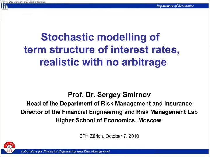
Stochastic modelling of term structure of interest rates, realistic with no arbitrage Prof. Dr. Sergey Smirnov Head of the Department of Risk Management and Insurance Director of the Financial Engineering and Risk Management Lab Higher School
Stochastic modelling of term structure of interest rates, realistic with no arbitrage Prof. Dr. Sergey Smirnov Head of the Department of Risk Management and Insurance Director of the Financial Engineering and Risk Management Lab Higher School of Economics, Moscow ETH Zürich, October 7, 2010
About Lab • The Financial Engineering & Risk Management Lab (FERMLab) was founded in March 2007 within the Department of Risk Management and Insurance of State University – Higher School of Economics. • The Lab’s mission is to promote the studies in modern financial engineering, risk management and actuarial methods both in financial institutions, such as banks, asset managers and insurance companies, and in non- financial enterprises. 2
Lab Team • Smirnov Sergey , PhD, Director of FERMLab; Head of Department of Risk-Management and Insurance; PRMIA Cofounder, Member of Education Committee of PRMIA; Vice-Chairman of European Bond Commission; Member of Advisory Panel of International Association of Deposit Insurers. • Sholomitski Alexey , PhD, Deputy Director of Laboratory for Financial Engineering and Risk Management; Deputy Head of Department of Risk-Management and Insurance. Actuarial science. • Kosyanenko Anton , MS,MA. Data filtering and augmentation.. • Lapshin Victor , MS. Term structure of interest rate modelling . • Naumenko Vladimir , MA. Market microstructure and liquidity research. 3
Key Lab Activities • Accumulation of financial and economics data required for empirical studies. • Empirical studies of the financial markets’ microstructure. • Development of structured financial products pricing and contingent liability hedging models. • Risk evaluation and management based on quantitative models • Actuarial studies for insurance and pensions applications. • Familiarization with and practical application of data analysis and modeling software. 4
Dealing with term structure of interest rates 5
Instruments • Term structure of interest rates can be constructed for different market instruments: bonds, interest rate swaps, FRA, etc. • In this presentation we consider only bond market as a source of information 6
Classification • By information used: – Snapshot methods. – Dynamic methods. • By a priori assumptions: – Parametric methods. – Nonparametric (spline) methods.
Some Approaches • Static methods - yield curve fitting – Parametric methods (Nelson-Siegel, Svensson) – Spline methods (Vasicek-Fong, Sinusoidal- Exponential splines) • Dynamic methods (examples) – General affine term structure model – HJM Markov evolution of forward rates
A Priori Assumptions • Incomplete and poor available data cannot be treated without additional assumptions. • Different assumptions lead to different problem statements and therefore to different results. • Often assumptions are chosen ad hoc, without economic interpretation 9
The Data • Available data: bonds, their prices, possibly bid-ask quotes. • Difficulties with observed data: – coupon-bearing bonds; – few traded bonds, – different credit quality and liquidity. 10
Term structure descriptions • Discount function • After a convention of mapping discount function to interest rates for different maturities is fixed: – Zero coupon yield curve – Instantaneous forward curve 11
Convenient compounding convention • Continuous compounding: = − d t ( ) exp[ t y t ( )] • Instantaneous forward rates: = ∫ 1 t y t ( ) r t dt ( ) t 0
Snapshots (static fitting) 13
Usual assumptions • Bonds to be used for determining yield curve are of the same credit quality, • All instruments have approximately the same liquidity. • A method using bonds of different credit quality for construction of risk-free zero coupon in Euro zone was propose by Smirnov et al (2006), see www.effas-ebc.org 14
Data treatment • Bond prices at the given moment. • Bid/Ask quotes at the given moment. • Other parameters: volumes, frequencies etc. • Bond price is assumed to be approximately equal to present value of promised cash flows: n ≈ ∑ P d t F ( ) k i i k , = i 1
The Problem = • Zero-coupon bonds: P N d t ( ) k k k − = r ( t ) t d ( t ) e ∑ = n ≈ • Coupon-bearing bonds: P F d ( t ) k i , k i i 0 P ≈ = Fd d d ( i t ) i • The system is typically underdetermined. • Discount function values are to be found in intermediate points. • Mathematically the problem is ill-posed 16
Different Approaches • Assumptions on a specific parametric form of the yield curve (parametric methods) • Assumptions on the degree of the smoothness (in some sense) of the yield curve (spline methods). 17
The term structure of interest rates estimation by different central banks BIS Papers No 25 October 2005 “Zero-coupon yield curves: technical documentation” Mainly parametric methods are used
Parametric methods of yield curve fitting Svensson ( 6 parameters) Instantaneous forward rate is assumed to have the following form: Nelson-Siegel (4 parameters) is a special case of Svensson with Assuming specific functional form for yield curve is arbitrary and has no economic ground
Nonparametric methods • Usually splines • Flexibility • Sensibility • Possibility of smoothness/accuracy control
The preconditions 1. Approximate discount function should be decreasing (i.e. forward rates should be non-negative) with initial value equal to one, and positive. 2. Approximate discount function should be sufficiently smooth. 3. Corresponding residual with respect to observed bond prices should be reasonably small. 4. The market liquidity is taken into account to determine the reasonable accuracy, e.g. the residual can be related to the size of bid-ask spreads. 21
Problem statement ensuring positive forward fates • Select the solution in the form: ⎡ ⎤ t ∫ = − τ τ 2 d t ( ) exp f ( ) d ⎢ ⎥ ⎣ ⎦ 0 • Select the degree of non-smoothness: T f ∫ ′ τ τ → 2 ( ) d min 0 • Minimize conditionally the residual: 2 ⎛ ⎞ N n ⎡ ⎤ ∑ ∑ t T ∫ ∫ ′ − τ τ − + α τ τ → i 2 2 w exp f ( ) d F P f ( ) d min ⎜ ⎟ ⎢ ⎥ ⎣ ⎦ k i k , k ⎝ ⎠ 0 0 f = = k 1 i 1 22
The semi-analitical solution Smirnov & Zakharov (2003): f(t) is a spline of the following form: ⎧ λ − + − λ − λ > C exp{ ( t t )} C exp{ ( t t )}, 0 − − 1 k k 1 2 k k 1 k ⎪ ⎪ = − λ − + − λ − λ < f t ( ) C sin( ( t t )) C cos( ( t t )), 0, ⎨ − − 1 k k 1 2 k k 1 k ⎪ − + λ = C t ( t ) C , 0 ⎪ − ⎩ 1 k 1 2 k ′ ′ ∈ − = + − = + t [ t ; ] t f t ( 0) f t ( 0), f t ( 0) f t ( 0) − k 1 k k k k k 23
History can be useful • Consider to consecutive days, when short term bonds are not traded (or quoted the second day:
Working with missing data 25
Approach • Data history accumulation • Filtration. • Data augmentation. • Application of fitting algorithms. 26
2 x ˆ = − T 1 ξ 2 0 Filters • Value level filter. • Value change filter. • Relative position of trade price compared to market quotes. • Liquidity filter (number of deals, turnover). 27
Relative position of trade price compared to market quotes 28
“Missing” data density 29
Overall trades volume 30
Bayesian estimation approach Posterior Prior density density Likelihood function - Multivariate parameter (random) - Observable data 31
Markov Chain Monte-Carlo X - Complete dataset (observable all +unobservable) = X ( X , X ) X - observable data all obs mis obs X - unobservable data mis θ p ( | X ) - “Complex” distribution obs θ p ( | X , X ) - “Simple” distribution obs mis 32
Markov Chain Monte-Carlo Imputation Step Generating missing data θ − ( ) t ( t 1) X ~ p X ( | X , ) mis mis obs Posterior Step Generating posterior distribution parameters θ θ ( ) t ( ) t ~ p ( | X , X ) obs mis Markov Chain θ θ ⎯⎯ → θ (1) (1) (2) (2) d ( X , ),( X , ),... p X ( , | X ) mis mis mis obs 33
ЕМ algorithm (industry standard) Filling missing data with conditional expectations ⎧ ∈ o y , y y , ij ij i ⎧ ⎪ ∈ o ∈ o 0 , y y и y y , ⎪ = old y ij i ik k ⎨ ⎛ ⎞ n = old c ( ) ⎨ ∑ ij θ ∈ ⎜ o old ⎟ u E y y , , y y ; ⎪ ijk θ o old cov y , y y , , в противном случае . ⎪ ij ij i ⎩ ⎝ ⎠ ⎩ ij ik = i 1 Recompute posterior distribution modes 1 n ∑ µ new = old = y , j 1 ,..., d j ij n = i 1 ⎛ ⎞ 1 n ∑ σ new = ⎜ old ⋅ old + old ⎟ − µ new µ new = y y c , j , k 1 ,..., d jk ij ik ijk j k n ⎝ ⎠ = i 1 Modes of joint posterior distribution of parameters and missing data 34
Parameters evaluation results (correlation coefficients) 35
Stochastic Evolution 36
Recommend
More recommend
Explore More Topics
Stay informed with curated content and fresh updates.
