Real-Time Motion Planning and Autonomous Driving Jeffrey - PowerPoint PPT Presentation
Real-Time Motion Planning and Autonomous Driving Jeffrey Ichnowski What is Real-Time Motion Planning? 1 st floor vs. 2 nd floor Motion planning with a hard real-time constraint. temporally correct T i = ( i , p i , e i , D i )
Real-Time Motion Planning and Autonomous Driving Jeffrey Ichnowski
What is Real-Time Motion Planning? 1 st floor vs. 2 nd floor Motion planning with a hard real-time constraint. temporally correct T i = ( φ i , p i , e i , D i )
Example Real-Time Motion Planning System T v T c T p Sense Plan Move (e.g., vision) (controller)
Problems with Motion Planning in a Real-Time System motion planning P-SPACE hard EXPSPACE ? exponential in dimensions = EXPTIME ? = PSPACE uncountably infinite ? = NP state spaces ? = P ? = NL [Image source: wikipedia]
Real-Time Motion Planning In the general case: impossible.
Precompute Motion Plan Extremely popular option. • Allows arbitrarily long computation • Asymptotically feasible algorithms • Asymptotically optimal algorithms Is this real-time? yes and no.
Real-time Motion Planning Problem Time-bounded computation Responsive a dynamic environment (moving obstacles, goals, new data)
Collision Avoidance • Reformulation of path planning into collision avoidance. • Potential fields • Real-time ✓ • Problem: gets stuck in local minima [Khatib 1986]
Anytime Planners • Incrementally build a planning tree • May be stopped at anytime • Example: RRT, RRT* • Real-time? • Reactivity: rapid re-planning + some luck [Image source: Ichnowski 2013]
Roadmap Planners • Pre-computes a roadmap (connectivity of freespace) • Motion plan = graph search • Real-time? • Example: PRM • Reactivity must come from another task. [Image source: LaValle 2006]
Grid/Lattice Planners 1. Discretize space 2. Plan in the discretized space Often done with A* or variant. Weighted A*: reduced plan optimality & compute time κ δ D* is reverse A* + keep data for next compute cycle [Image source: Pivtoraiko 2006] δ
A* • Provably optimal • What if graph changes during the search? (e.g., dynamic environment) • O(b d ) d = solution length, b = branching factor. (polynomial if search space is tree*)
Real-Time Heuristic Search 𝛽 -Pruning Minimin + • Assign α = min x ∈ S f ( x ) 1. Depth-limited horizon search • Prune search when 2. A* metric frontier ( S ) f ( x ) ≥ α f ( x ) = g ( x ) + h ( x ) 3. Take step towards best frontier node 4. repeat. [Korf 1988]
Real-Time A* • Use Minimin w/ 𝛽 -Pruning in “planning mode” • RTA* used in execution. RTA*: At , what is ? x i +1 x i g ( x 0 ) + h ( x 0 ) x i +1 = argmin 1. Choose x 0 2 neighbors of x i g ( x 0 ) + h ( x 0 ) 2. Store second best for x i [Korf 1988]
Partitioned-Learning RTA* • Start w/ RTA* (depth-limited search) • Take step towards best path • “Learn” h(x) of all frontier • Split f(x) into dynamic and AUTHOR COPY static components f ( x ) = g s ( x ) + g d ( x ) + h s ( x ) + h d ( x ) [Cannon et. al. 2014]
Real-Time R* (RTR*) R* ≈ RRT + A* RTR* • fixed # of node expansions • choose best frontier node (path and min g(x) + h(x)) • geometric expansion limits for difficult nodes • path reuse [Cannon et. al. 2014] AUTHOR COPY
Hard-Real-Time Rapidly-exploring Randomized Trees procedure HRT_PLANNER x target t_next = current_time() loop x init x near yield until t_next t_next = t_next + T_p Execution period B = updated map q_init = current vehicle state q_goal = current goal states T = BUILD_RRT(q_init, q_goal, n) solution or path = EXTRACT_PATH(T) “safe” number of samples publish path path (WCET analysis) [Walker, 2011]
Source Code WCET Instr. Source Code Estimation Compilation Flow Facts Tool-chain Object Code Execution Execution Trace Control Flow Graph Basic Block Exec. Times Integer Linear Program WCET [Walker, 2011]
900 Predicted WCET Empty Observed Exection Time 800 700 Execution Time (ms) 600 Workspace 500 400 300 200 100 0 500 1000 1500 2000 Tree Size (#nodes) [Walker, 2011]
900 Predicted WCET Infeasible Observed Exection Time 800 700 Execution Time (ms) 600 Workspace 500 400 300 200 100 0 500 1000 1500 2000 Tree Size (#nodes) [Walker, 2011]
900 Predicted WCET Obstructed Observed Exection Time 800 700 Execution Time (ms) 600 Workspace 500 400 300 200 100 0 500 1000 1500 2000 Tree Size (#nodes) [Walker, 2011]
Solution Probability Probability of finding a solution (Empty Workspace) Probability of finding a solution (Obstructed Workspace) 1.0 1.0 0.8 0.8 0.6 0.6 Probability Probability Planner - RRT Planner - RRT Planner - RRT-LPM Planner - RRT-LPM 0.4 0.4 0.2 0.2 0.0 0.0 200 400 600 800 1000 1200 1400 1600 1800 2000 200 400 600 800 1000 1200 1400 1600 1800 2000 Search Tree size (vertices) Search Tree size (vertices) [Walker, 2011]
Real-Time Motion Planning for Autonomous Vehicles Reduce dimensionality of planning problem. Typically around 4: e.g., (x, y, 𝜄 , v) Discretization and sampling-based approaches
DARPA Urban Challenge 1st place: Tartan Racing (CMU) local planner at 10 Hz fixed lattice planner at 10 Hz (nominally) • Difficult scenarios take “up to a couple of seconds” (motivation for their pre-planning) • Anytime planner example: first solution in 100 ms, optimal at 650 ms. • Time for replanning “few ms” for small adjustments to “few seconds” for drastically different trajectories [Likhachev 2008] & [Ferguson 2008]
DARPA Urban Challenge 1st place: Tartan Racing (CMU) solution found <100 ms optimal solution solution < 650 ms improved Anytime planner behavior [Likhachev, et. al. 2008]
DARPA Urban Challenge 1st place: Tartan Racing (CMU) Effect of heuristic on A* search States Time Expanded (seconds) 2,019 0.06 h 26,108 1.30 h 2 D Implies much 124,794 3.49 h fsh higher WCET [Likhachev, et. al. 2008]
DARPA Urban Challenge 1st place: Tartan Racing (CMU) “One of the important lessons learned during the development of this system was that it is often extremely beneficial to exploit prior, offline processing to provide efficient online planning performance.” – Ferguson, Howard, and Likhachev
DARPA Urban Challenge 2nd place: Stanford Racing • Sensors at 10 Hz Grid: 160 m ⨉ 160 m ⨉ 360° • RNDF ¹ editor at 10 Hz Resolution of 1 m ⨉ 1 m ⨉ 5° • Full replanning: 50 to 300 ms 1. hybrid A* (unnatural swerves) 2. conjugate-gradient descent smooth (0.5 m) 3. interpolation (5 to 10 cm) ¹ route network definitions file [Montemerlo et. al. 2009] [Dolgov et. al. 2010]
DARPA Urban Challenge 2nd place: Stanford Racing Hybrid A* CG Smoothed [Dolgov et. al. 2010]
DARPA Urban Challenge 2nd place: Stanford Racing [Dolgov et. al. 2010]
DARPA Urban Challenge 4th place: MIT • Drivability map updated 10 Hz • Controller ran at 25 Hz • RRT at 10 Hz • 700 samples per second [Kuwata, et. al. 2009]
DARPA Urban Challenge 4th place: MIT procedure RRT_execution_loop repeat update vehicle states and env while ( t < t 0 + ∆ t ) hard real-time EXPAND_RRT_TREE() constraint repeat { = EXTRACT_BEST_SAFE_PATH() τ “take if NO safe path appropriate E-STOP! & restart action” } until (clear( x ) ∀ x ∈ τ ) send to controller τ [Kuwata, et. al. 2009]
DARPA Urban Challenge 4th place: MIT Lane following on a curve at 22.4 mph. The green dots are safe stopping nodes. [Kuwata, et. al. 2009]
DARPA Urban Challenge finalist: AnnieWay (KIT) • DNF. Froze at entrance to traffic circle (who doesn’t their first time?) Software exception during mode switch Caught by error handler, and left hanging Not observable by watchdog module. • One of the few cars that drove collision-free • One of the authors Matthias Goebl from Institute for Real- Time Computer Systems, Technical University of Munich [Kammel, et. al. 2008]
DARPA Urban Challenge finalist: AnnieWay (KIT) • Multi-level control: A. Mission planning B. Maneuver planning C. Collision avoidance { Car and Kernel Environment w/ RT* D. Reactive layer w/ 1m safety buffer car convolution E. Vehicle control • Motion planning on discretized grid of 3D configuration space using A*. • Convolutional filters used to precompute free C-space. [Kammel, et. al. 2008]
Conclusions • Real-time motion planning difficult • No guarantees on solution • Multiple levels of planning • Time-bounded computation • Generate “safe routes” • Keep around information between task cycles
Thank you
Recommend
More recommend
Explore More Topics
Stay informed with curated content and fresh updates.
