Raytracer 2 We start with some bits we missed in the previous - PowerPoint PPT Presentation
Raytracer 2 We start with some bits we missed in the previous lecture General camera in word coordinates (we positioned in (0,0,0) in the previous slides Computing refraction term without trigo (by means of dot products) Some
Raytracer 2 • We start with some bits we missed in the previous lecture – General camera in word coordinates (we positioned in (0,0,0) in the previous slides – Computing refraction term without trigo (by means of dot products) • Some ray tracer acceleration techniques • Overview of the basic version of the algorithm – To make your life a bit easier during the ex.
Eye LUV Coordinates l = (lookat - eye )/|| (lookat - eye )|| v = ( l × up )/||( l × up )|| u = v × l up u eye l v lookat (Gram-Schmidt Ortho-normalization)
Pixels in World Coords - a v • aspect ratio a = w / h -u • focal length d = 1/tan(fovy/2) ll d l fovy ll = eye + d l – a v – u eye for (j = 0; j < VRES; j++) { for (j = 0; j < VRES; j++) { for (i = 0; i < HRES; i++) { for (i = 0; i < HRES; i++) { p = ll + 2a v (double)i/HRES + 2 u p = ll + 2a v (double)i/HRES + 2 u (double)j/VRES; (double)j/VRES; color = TraceRay(Ray( eye , p - eye )); color = TraceRay(Ray( eye , p - eye )); plot(i,j,color); plot(i,j,color); } } } }
n cos θ i n - i Refract (using dot products) θ i cos θ i n i Snell’s Law: η i sin θ i = η t sin θ t m Let η = η i / η t = sin θ t / sin θ i Let m = (cos θ i n - i ) / sin θ i θ t Then… t = ? t = sin θ t m - cos θ t n - n = (sin θ t / sin θ i ) (cos θ i n - i ) - cos θ t n = ( η cos θ i - cos θ t ) n - η i θ = − θ 2 cos 1 sin ( ) t t = η ⋅ − − η − ⋅ − η = − η θ 2 2 2 2 ( ) 1 ( 1 ( ) ) 1 sin t n i n i n i i Can be negative for grazing Ray refract(Ray r) { Can be negative for grazing Ray refract(Ray r) { angles when η >1, say when angles when η >1, say when double ni = dot(n,-r.d); double ni = dot(n,-r.d); going from glass to air, double eta = current_index/new_index; going from glass to air, double eta = current_index/new_index; resulting in total internal return Ray((x,eta*ni - sqrt(1 - eta*eta*(1-ni*ni)))*n + eta*r.d); resulting in total internal return Ray((x,eta*ni - sqrt(1 - eta*eta*(1-ni*ni)))*n + eta*r.d); reflection (no refraction). } reflection (no refraction). }
Ray Tracing Acceleration
Bounding Volume Hierarchies The basic concept of a bounding volume hierarchy is a complex object in a � hierarchy of simpler ones This works much like the hierarchical culling we looked at in the scene � graph lecture For example, if one were using spheres as their bounding volume, we could � enclose the entire scene in one big sphere Within that sphere are several other spheres, each containing more � spheres, until we finally get to the bottom level where spheres contain actual geometry like triangles To test a ray against the scene, we traverse the hierarchy from the top level � When a sphere is hit, we test the spheres it contains, and ultimately the � triangles/primitives within In general, a bounding volume hierarchy can reduce the ray intersection � time from O( n ) to O(log n ), where n is the number of primitives in the scene This reduction from linear to logarithmic performance makes a huge � difference and makes it possible to construct scenes with millions of primitives
Sphere Hierarchies The sphere hierarchy makes for a good example of the concept, but in � practice, sphere hierarchies are not often used for ray tracing One reason is that it is not clear how to automatically group an arbitrary set � of triangles into some number of spheres, so various heuristic options exist Also, as the spheres are likely to overlap a lot, they end up triggering a lot � of redundant intersection tests
Octrees The octree starts by placing a cube around the entire scene � If the cube contains more than some specified number of primitives � (say, 10), then it is split equally into 8 cubes, which are then recursively tested and possibly resplit The octree is a more regular structure than the sphere tree and � provides a clear rule for subdivision and no overlap between cells This makes it a better choice usually, but still not ideal � Note: the drawing is actually a 2D quadtree , but the octree is a 3D extension of this concept
KD Trees The KD tree starts by placing a box (not necessarily a cube) around the entire scene � If the box contains too many primitives, it is split, as with the octree � However, the KD tree only splits the box into two boxes, that need not be equal � The split can take place on the x, y, or z place at some arbitrary point within the box � This makes the KD tree a little bit more adaptable to irregular geometry and able to � customize a tighter fit In general, KD trees tend to be pretty good for ray tracing � Their main drawback is that the tree depth can get rather deep, causing the ray � intersection to spend a lot of time traversing the tree itself, rather than testing intersections with primitives
BSP Trees The BSP tree ( binary space partitioning ) is much like the KD tree in � that it continually splits space into two (not necessarily equal) halves Unlike the KD tree which is limited to xyz axis splitting, the BSP tree � allows the splitting plane to be placed anywhere in the volume and aligned in any direction This makes it a much more difficult problem to choose the location � of the splitting plane, and so many heuristics exist In practice, BSP trees tend to perform well for ray tracing, much like � KD trees
Uniform Grids One can also subdivide space into a uniform grid, instead of hierarchically � This is fast for certain situations, but gets too expensive in terms of memory � for large complex scenes It also tends to loose its performance advantages in situations where � primitives have a large variance in size and location (which is common) As a result, they are not really a practical general purpose acceleration � structure for ray tracing, although they are useful in certain situations
Hierarchical Grids � One can also make a hierarchical grid � Start with a uniform grid, but subdivide any cell that contains too many primitives into a smaller grid � An octree is an example of a hierarchical grid limited to 2x2x2 subdivision � A more general hierarchical grid could support subdivision into any number of cells � Hierarchical grids tend to perform very well in ray tracing, especially for highly detailed geometry of relatively uniform size (such as the triangles in a tessellated surface)
Ray Tracing Acceleration Techniques Acceleration Techniques Faster Fewer Rays Generalized Rays Intersections Faster ray-object Fewer ray-object intersections intersections Adaptive Volume Beam tracing Bounding tree-depth hierarchies volumes Cone tracing Adaptive Spatial Efficient Pencil tracing sampling subdivision surfaces Directional techniques
Ray tracer pseudo-code
Generating Rays � Trace a ray for each pixel in the image plane renderImage(){ for each pixel i, j in the image ray.setStart(0, 0, 0); // r o ray.setDir ((.5 + i) * tan(fov x )* 2 / m, (.5 + j) * tan(fov y )* 2 / n, 1.0); // r d ray.normalize(); image[i][j] = rayTrace(ray); }
Recursive ray evaluation rayTrace(ray) { hitObject(ray, p, n, triangle); color = object color; if(object is light) return(color); else return(lighting(p, n, color)); }
Finding Intersections � Check all triangles, keep the closest intersection hitObject(ray) { for each triangle in scene does ray intersect triangle? if(intersected and was closer) save that intersection if(intersected) return intersection point and normal }
Calculating surface color lighting(point) { color = ambient color; for each light if(hitObject(shadow ray)) color += lightcolor * dot(shadow ray, n); color += rayTrace(reflection) * pow(dot(reflection, ray), shininess); return(color); }
Putting It All Together � The main program main() { triangles = readTriangles(); image = renderImage(triangles); writeImage(image); }
Recommend
More recommend
Explore More Topics
Stay informed with curated content and fresh updates.
