RANS-CFD code with a k- turbulence closure F. VENDEL Florian - PowerPoint PPT Presentation

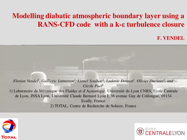
Modelling diabatic atmospheric boundary layer using a RANS-CFD code with a k- ε turbulence closure F. VENDEL Florian Vendel 1 , Guillevic Lamaison 1 , Lionel Soulhac 1 , Ludovic Donnat 2 , Olivier Duclaux 2 , and Cécile Puel 2 1) Laboratoire de Mécanique des Fluides et d’Acoustique, Université de Lyon CNRS, Ecole Centrale de Lyon, INSA Lyon, Université Claude Bernard Lyon I, 36 avenue Guy de Collongue, 69134 Ecully, France 2) TOTAL, Centre de Recherche de Solaize, France

Introduction Context • Modelling of pollutant dispersion over industrial areas implies the description of the stratified surface layer flow and its interaction with buildings or complex obstacles • Better computers performances make it possible today to simulate this flow using CFD models and RANS equations (Fluent, Phoenics, StarCD…) • But, generally standard parameterization implemented in these commercial models are not really adapted so as to represent the atmosphere So the question is : how to parameterize the atmospheric processes, particularly thermal stratification in a RANS-CFD code? 2

Introduction CFD modelling of the SBL in the literature • Application of CFD models in neutral stability conditions • Richards P.J. and Hoxey R.P., 1993 • Blocken B. and al., 2007 • Hargreaves D.M. and Wright N.G., 2007 • Application in stable or unstable stability conditions (less studied) • Duynkerke P.G., 1988 : modification of the k- ε model constants to match the physical characteristic of atmospheric surface layer in neutral and stable conditions • Huser A. and al., 1997 : inlet turbulence profiles does not maintain with distance (turbulence increase in stable stratification) • Pontiggia M. and al., 2009 : add a source term in turbulent dissipation rate e equation 3

Introduction Main points to model • To model a surface boundary layer with RANS-CFD codes, we focus on two main points : Top boundary conditions Equations solved : Inlet boundary • Momentum equations Outflow boundary conditions conditions • Energy equation • Turbulence closure Ground boundary conditions 4

Introduction Some questions unsolved • Equations solved : • Which set of equations models properly the flow and the turbulence for a diabatic surface layer ? How to treat the inconsistency between the k and e profiles • (stable/unstable conditions) and the conservation equations ? • Boundary conditions : • How to describe the pressure profile in order to define appropriate downwind boundary conditions for stable and unstable cases ? • How to describe the inlet profiles to represent diabatic surface layer ? • How to impose a constant flux of momentum and energy with the altitude (surface boundary layer assumption) ? 5

Summary 1. Reference model of the surface boundary layer 2. Consistency with k and e equations 3. Parameterization of a diabatic surface layer in a RANS CFD simulation 6

1. – Reference model of the surface boundary layer Surface boundary layer assumptions • The flow is oriented along the x direction and the mean vertical  w  velocity is equal to zero : v 0 (1) • The vertical turbulent fluxes (Reynolds stresses and heat flux) are constant with respect to altitude (Garratt J.R., 1992) :     2 u ' w ' cste u *  (2)  H       0 w ' ' cste u  * *  C  0 p • The Monin-Obukhov similarity theory predicts that the dimensionless gradient of velocity and potential temperature only depends on z/L MO (Garratt J.R., 1992) :      z u     m    3  u z C u * z 0 p 0 *      where and (3) L    MO   z   L gH    MO 0 7  h    z *

1. – Reference model of the surface boundary layer Surface boundary layer assumptions • The turbulence satisfies a local equilibrium within the surface layer (Tennekes, H. and Lumley, J. L., 1972) :   u    P u ' w ' shear TKE production  (4)  z   g  B  e     P B w ' ' thermal TKE production / destructio n with   0  e  turbulent dissipatio n rate   • Influence of buoyancy effects in the momentum equation can be taken into account using Boussinesq approximation (the density is constant except in the buoyancy term of the momentum equation) :     cste (5) 0 1             ( ) g ( ) g with for an ideal gas (6) 0 0 0  8 0

1. – Reference model of the surface boundary layer Conservation equations • When using the precedent assumptions, the Reynolds Averaged Navier-Stokes (RANS) conservation equations for the mass, horizontal momentum and energy are verified and the vertical momentum equation reduces to :  P            P P P gz ( ) g (7) with 0 0 abs 0 0  z Where is defined as difference between absolute and hydrostatic pressure. P • Integration of this equation will give the vertical profile of in a P stable boundary layer. •    is constant for the neutral case, where ( z ) P 0 9

1. – Reference model of the surface boundary layer k- ε turbulence closure • In order to model the turbulence fluxes, we use in this work a k- ε turbulent closure :   u   ' ' u w K  m   k ² K z K m   m  C K (8) with  and   e h  Pr  '   t w ' K  h   z Where k is the turbulent kinetic energy, ε the turbulent dissipation rate and K m and K h are the turbulent diffusivity of momentum and heat. • k and ε are given by two conservation equations (steady surface layer) :     K k      e  m P B 0 (9)   Where D is the diffusion term      z z k      D     e e e K P ²      m C C 0   e e (10) 1 2      z z k k e 10

1. – Reference model of the surface boundary layer k- ε turbulence closure • Focus on the turbulent dissipation rate equation :     e e e K P ²      m 0 C C   e e    1 2   z z k k e • No term for the buoyancy effects (Duynkerke P .G., 1988) • The use of k- ε model requires values for the parameters C µ , σ k , σ ε , C ε 1 , C ε 2 • For simulating realistic atmospheric values of the TKE in the surface   layer (        Garratt J. R., 1992 ), we use the 2 2 2 2 k 1 2 5 . 5 u u v w * modified constant set proposed by Duynkerke P . G., 1998 .  k  e c  c e 1 c e 2 0.033 1.0 2.38 1.46 1.83 Table 1. Duynkerke constants for the k- ε model 11

    2  u ' w ' cste u *  1. – Reference model of the surface        w ' ' cste u * * (2) boundary layer    z u       Set of equations for the vertical profiles  m  u z *      z      • Integration of (3) gives classical logarithmic velocity and temperature  h    z * profiles : (3)        u       * z   u z ln     B  e    m   z  P 0     (11) with               * z   z ln      u 0    h  z     t P u ' w '    z Where ψ m et ψ h are the integrated universal functions of the Monin-Obukhov theory  g    ' ' B  w  •  Integrations of (7) using the precedent relations (11) provides : 0 (4) z         g         0 * z    P z ln dz   P    h (12)         z  ( ) g t 0  0 0 0 z • With equation (2), (3), (4), one can derive the profile of ε : (7)   u      3  u ' w ' K   u    m e      * z  1    z (13)  m      z   m   '   w ' K  h •   Combining equations (2), (8), (13) gives the profile of k : z with 2  k ²   u K m    * C 1 k z    (14) e   C µ m and    u z • 12  Equations (8), (13), (14) provide the profile K m : * K K z (15)    m K m   h Pr m t (8)