Random Walks Conditioned to Stay Positive Bob Keener Let S n be a - PowerPoint PPT Presentation

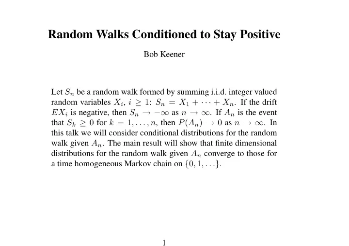
Random Walks Conditioned to Stay Positive Bob Keener Let S n be a random walk formed by summing i.i.d. integer valued random variables X i , i ≥ 1 : S n = X 1 + · · · + X n . If the drift EX i is negative, then S n → −∞ as n → ∞ . If A n is the event that S k ≥ 0 for k = 1 , . . . , n , then P ( A n ) → 0 as n → ∞ . In this talk we will consider conditional distributions for the random walk given A n . The main result will show that finite dimensional distributions for the random walk given A n converge to those for a time homogeneous Markov chain on { 0 , 1 , . . . } . 1

Exponential Families Let h denote the mass function for an integer valued random variable X under P 0 . Assume that E 0 X = � xh ( x ) = 0 , and define e ψ ( ω ) = E 0 e ωX = � e ωx h ( x ) . (1) x Then f ω ( x ) = h ( x ) exp[ ωx − ψ ( ω )] , is a probability mass function whenever ω ∈ Ω = { ω : ψ ( ω ) < ∞} .. Let X, X 1 , . . . be i.i.d. under P ω with marginal mass function f ω . Differentiating (1), ψ ′ ( ω ) e ψ ( ω ) = � xe ωx h ( x ) , x and so E ω X = ψ ′ ( ω ) . Similarly, Var ω ( X ) = ψ ′′ ( ω ) . Note that since ψ ′′ > 0 , ψ ′ is increasing, and since ψ ′ (0) = E 0 X = 0 , ψ ′ ( ω ) < 0 when ω < 0 . 2

Classical Large Deviation Theory Exponential Tilting: Let S n = X 1 + · · · + X n and X n = S n /n . Since X 1 , . . . , X n have joint mass function � n n � � � � � h ( x i ) exp[ ωx i − ψ ( ω )] = h ( x i ) exp[ ωs n − nψ ( ω )] , i =1 i =1 E ω f ( X 1 , . . . , X n ) = E 0 f ( X 1 , . . . , X n ) exp[ ωS n − nψ ( ω )] . and In particular, P ω ( S n ≥ 0) = e − nψ ( ω ) E 0 [ e ωS n ; S n ≥ 0] . def For notation, E [ Y ; A ] = E [ Y 1 A ] . Using this, it is easy to argue that if ω < 0 , 1 P ω ( S n ≥ 0) = e − nψ ( ω ) × e o ( n ) . n log P ω ( S n ≥ 0) → − ψ ( ω ) , or Also, for any � > 0 , P ω ( X n > � | X n ≥ 0) → 0 , as n → ∞ . [For regularity, need 0 ∈ Ω o .] 3

Refinements Local Central Limit Theorem: If the distribution for X is lattice with span 1, then as n → ∞ , � P 0 [ S n = k ] ∼ 1 / 2 πnψ ′′ (0) . Using this, for ω < 0 , P ω ( S n ≥ 0) = e − nψ ( ω ) E 0 [ e ωS n ; S n ≥ 0] ∞ e ωk � ∼ e − nψ ( ω ) � 2 πnψ ′′ (0) k =0 e − nψ ( ω ) = , � (1 − e ω ) 2 πnψ ′′ (0) and P ( S n = k | S n ≥ 0) → (1 − e ω ) e ωk , the mass function for a geometric distribution with success probability e ω . 4

Goal, Sufficiency, and Notation Let τ = inf { n : S n < 0 } and note that τ > n S j ≥ 0 , j = 1 , . . . , n. if and only if Goal: Study the behavior of the random walk given τ > n for large n . Sufficiency: Under P ω , the conditional distribution for X 1 , . . . , X n given S n does not depend on ω . New Measures: Under P ( a ) ω , the summands X 1 , X 2 , . . . are still i.i.d. with com- mon mass function f ω , but S n = a + X 1 + · · · + X n . Finally, P ( a,b ) denotes conditional probability under P ( a ) given S n = b . Under n ω this measure, S k goes from a to b in n steps. 5

Positive Drift If ω > 0 , then E ω X > 0 . In this case, P ( a ) ω ( τ = ∞ ) > 0 , and conditioning on τ = ∞ is simple. For x ≥ 0 , ω ( S 1 = x | τ = ∞ ) = P ( a ) ω ( S 1 = x, τ = ∞ ) P ( a ) P ( a ) ω ( τ = ∞ ) ω ( S 1 = x ) P ( x ) ω ( τ = ∞ ) = P ( a ) . P ( a ) ω ( τ = ∞ ) Given τ = ∞ , the process S n , n ≥ 0 , is a random walk, and the conditional transition kernel is an h -transform of the original transition kernel for S n . 6

Simple Random Walk If X i = ± 1 with p = P ω ( X i = 1) , q = 1 − p = P ω ( X i = − 1) , and ω = 1 2 log( p/q ) , then S n , n ≥ 0 , is a simple random walk . Theorem: For a simple random walk, as n → ∞ , ( τ > n ) ∼ 2( a + 1)( b + 1) P ( a,b ) . n n Proof. By the reflection principle, P ( a ) ( τ < n, S n = b ) = P ( a ) ( S n = − b − 2) . 0 0 Dividing by P 0 ( S n = b ) (a binomial probability), � n + b − a � n − b + a � � ! ! P ( a,b ) 2 2 ( τ < n ) = ! . � n − a − b − 2 � n + a + b +2 n � � ! 2 2 Result follows from Stirling’s formula. � 7

Result for Simple Random Walks Let Y n , n ≥ 0 , be a Markov chain on { 0 , 1 , . . . } with Y 0 = 0 and transition matrix   0 1 0 0 0 · · · 1 / 4 0 3 / 4 0 0 · · ·     0 2 / 6 0 4 / 6 0 · · ·     0 0 3 / 8 0 5 / 8   . .   ... ... ... . . . . Theorem: For a simple random walk with p < 1 / 2 , P ω ( S 1 = y 1 , . . . , S j = y j | τ > n ) → P ( Y 1 = y 1 , . . . , Y j = y j ) as n → ∞ . 8

Proof: Let B = { S 1 = y 1 , . . . , S j = y j = y } with y 1 = 1 , y i ≥ 0 , and | y i +1 − y i | = 1 . Then ( B, τ > n ) = P 0 ( B, τ > n, S n = b ) P (0 ,b ) n P 0 ( S n = b ) (1 / 2) j P ( y,b ) n − j ( τ > n − j ) P 0 ( S n − j = b − y ) = P 0 ( S n = b ) ∼ 2( y + 1)( b + 1) . 2 j n Use this in b P (0 ,b ) � ( B, τ > n ) P ω ( S n = b ) n P ω ( B | τ > n ) = . b P (0 ,b ) � ( τ > n ) P ω ( S n = b ) n � 9

General Results For the general case, let Y n , n ≥ 0 , be a stationary Markov chain with Y 0 = 0 and P ( Y n +1 = z | Y n = y ) = P 0 ( X = z − y ) E ( z ) 0 ( z − S τ ) . E ( y ) 0 ( y − S τ ) Remark: the transition kernel for Y is an h -transform of the kernel for the random walk under P 0 . Theorem: For ω < 0 , P ω ( S 1 = y 1 , . . . , S k = y k | τ > n ) → P ( Y 1 = y 1 , . . . , Y k = y k ) as n → ∞ . Theorem: Let τ + ( b ) = inf { n : S n > b } . For ω < 0 , e bω E 0 S τ + ( b ) P ω ( S n = b | τ > n ) → . � ∞ k =0 e kω E 0 S τ + ( k ) 10

( τ > n ) , b of order √ n . Approximate Reflection : P ( a,b ) n Proposition: If 0 ≤ b = O ( √ n ) , 1 / √ n 2 b nψ ′′ (0) E ( a ) P ( a,b ) � � ( τ > n ) = 0 ( a − S τ ) + o . n Proof: Let g k denote the P 0 mass function for S k , and define L k ( x ) = P ( a,b ) ( S k = x ) = g n − k ( b − x ) g n ( − b − a ) n g n − k ( − b − x ) g n ( b − a ) . P ( a, − b ) ( S k = x ) n Then L k ( S k ) is dP ( a,b ) /dP ( a, − b ) restricted to σ ( S k ) or σ ( X 1 , . . . , X k ) , and n n P ( a,b ) ( τ ≤ n ) = E ( a, − b ) L τ ( S τ ) n n 1 / √ n � �� 2 b = E ( a, − b ) � 1 − nψ ′′ (0)( a − S τ ) + o . n Finish by arguing that E ( a, − b ) S τ → E ( a ) 0 S τ . � n 11

Approximate Reflection : P ( a,b ) ( τ > n ) , b of order one. n Corollary: As n → ∞ , 2 nψ ′′ (0) E ( a ) 0 ( a − S τ ) E ( b ) P ( a,b ) ( τ > n ) = 0 ( b − S τ ) + o (1 /n ) . n Proof: Take m = ⌊ n/ 2 ⌋ . Then ∞ ( τ > m ) P ( b,c ) � P ( a,b ) P ( a,b ) ( S m = c ) P ( a,c ) ( τ > n ) = n − m ( τ > n − m ) . n n m c =0 Result follows using the prior result since S m under P ( a,b ) is approximately n normal. � 12

References • Keener (1992). Limit theorems for random walks conditioned to stay positive. Ann. Probab. • Iglehart (1974). Functional central limit theorems for random walks con- ditioned to stay positive. Ann. Probab. • Durrett (1980). Conditioned limit theorems for random walks with neg- ative drift. Z. Wahrsch. verw. Gebiete • Bertoin and Doney (1992). On conditioning a random walk to stay non- negative. Ann. Probab. 13