Random triangulations coupled with an Ising model Laurent M enard - PowerPoint PPT Presentation
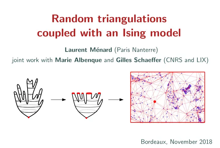
Random triangulations coupled with an Ising model Laurent M enard (Paris Nanterre) joint work with Marie Albenque and Gilles Schaeffer (CNRS and LIX) Bordeaux, November 2018 Outline 1. Introduction: 2DQG and planar maps 2. Local weak
Random triangulations coupled with an Ising model Laurent M´ enard (Paris Nanterre) joint work with Marie Albenque and Gilles Schaeffer (CNRS and LIX) Bordeaux, November 2018
Outline 1. Introduction: 2DQG and planar maps 2. Local weak topology 3. Adding matter: Ising model 4. Combinatorics of triangulations with spins 5. Local limit of triangulations with spins
2D Quantum Gravity? ”We have to develop an art of handling sums over [Polyakov 81] random surfaces . These sums replace the old fashioned (and extremely useful) sums over random paths .”
2D Quantum Gravity? ”We have to develop an art of handling sums over [Polyakov 81] random surfaces . These sums replace the old fashioned (and extremely useful) sums over random paths .” Sums over random paths: Feynman path integrals. Well understood question: Pick a, b ∈ R 2 , what does a random path γ : [0 , 1] → R 2 chosen ”uniformly at random” between all paths from a to b look like?
2D Quantum Gravity? ”We have to develop an art of handling sums over [Polyakov 81] random surfaces . These sums replace the old fashioned (and extremely useful) sums over random paths .” Sums over random paths: Feynman path integrals. Well understood question: Pick a, b ∈ R 2 , what does a random path γ : [0 , 1] → R 2 chosen ”uniformly at random” between all paths from a to b look like? Brownian motion!
2D Quantum Gravity? ”We have to develop an art of handling sums over [Polyakov 81] random surfaces . These sums replace the old fashioned (and extremely useful) sums over random paths .” Sums over random paths: Feynman path integrals. Well understood question: Pick a, b ∈ R 2 , what does a random path γ : [0 , 1] → R 2 chosen ”uniformly at random” between all paths from a to b look like? Brownian motion! Not so well understood question: What does a random metric on S 2 distributed ”uniformly” look like? Brownian surface?
2D Quantum Gravity? ”We have to develop an art of handling sums over [Polyakov 81] random surfaces . These sums replace the old fashioned (and extremely useful) sums over random paths .” Sums over random paths: Feynman path integrals. Well understood question: Pick a, b ∈ R 2 , what does a random path γ : [0 , 1] → R 2 chosen ”uniformly at random” between all paths from a to b look like? Brownian motion! Not so well understood question: What does a random metric on S 2 distributed ”uniformly” look like? Brownian surface? First idea: try discrete metric spaces (Donsker)
Planar Maps as discrete planar metric spaces Definition: A planar map is a proper embedding of a finite connected graph into the two-dimensional sphere (considered up to orientation-preserving homeomorphisms of the sphere).
Planar Maps as discrete planar metric spaces Definition: A planar map is a proper embedding of a finite connected graph into the two-dimensional sphere (considered up to orientation-preserving homeomorphisms of the sphere). = = � =
Planar Maps as discrete planar metric spaces Definition: A planar map is a proper embedding of a finite connected graph into the two-dimensional sphere (considered up to orientation-preserving homeomorphisms of the sphere). faces: connected components of the complement of edges p -angulation: each face is bounded by p edges = = � =
Planar Maps as discrete planar metric spaces Definition: A planar map is a proper embedding of a finite connected graph into the two-dimensional sphere (considered up to orientation-preserving homeomorphisms of the sphere). faces: connected components of the complement of edges p -angulation: each face is bounded by p edges
Planar Maps as discrete planar metric spaces Definition: A planar map is a proper embedding of a finite connected graph into the two-dimensional sphere (considered up to orientation-preserving homeomorphisms of the sphere). faces: connected components of the complement of edges p -angulation: each face is bounded by p edges
Planar Maps as discrete planar metric spaces Definition: A planar map is a proper embedding of a finite connected graph into the two-dimensional sphere (considered up to orientation-preserving homeomorphisms of the sphere). faces: connected components of the complement of edges p -angulation: each face is bounded by p edges This is a triangulation
Planar Maps as discrete planar metric spaces Definition: A planar map is a proper embedding of a finite connected graph into the two-dimensional sphere (considered up to orientation-preserving homeomorphisms of the sphere). 1 1 1 1 1 0 1 1 2 In blue, distances from M Planar Map: • V ( M ) := set of vertices of M • d gr := graph distance on V ( M ) • ( V ( M ) , d gr ) is a (finite) metric space
Planar Maps as discrete planar metric spaces Definition: A planar map is a proper embedding of a finite connected graph into the two-dimensional sphere (considered up to orientation-preserving homeomorphisms of the sphere). 1 1 1 1 1 0 1 1 2 In blue, distances from M Planar Map: • V ( M ) := set of vertices of M • d gr := graph distance on V ( M ) • ( V ( M ) , d gr ) is a (finite) metric space Rooted map: mark an oriented edge of the map
”Classical” large random triangulations Euler relation in a triangulation: number of edges / vertices / faces linked Take a triangulation of size n uniformly at random. What does it look like if n is large ? Two points of view: global/local, continuous/discrete
”Classical” large random triangulations Euler relation in a triangulation: number of edges / vertices / faces linked Take a triangulation of size n uniformly at random. What does it look like if n is large ? Two points of view: global/local, continuous/discrete Global : Rescale distances to keep diameter bounded [Le Gall 13, Miermont 13]: converges to the Brownian map . • Gromov-Hausdorff topology • Continuous metric space • Homeomorphic to the sphere • Hausdorff dimension 4 • Universality
”Classical” large random triangulations Euler relation in a triangulation: number of edges / vertices / faces linked Take a triangulation of size n uniformly at random. What does it look like if n is large ? Two points of view: global/local, continuous/discrete Local : Don’t rescale distances and look at neighborhoods of the root
”Classical” large random triangulations Euler relation in a triangulation: number of edges / vertices / faces linked Take a triangulation of size n uniformly at random. What does it look like if n is large ? Two points of view: global/local, continuous/discrete Local : Don’t rescale distances and look at neighborhoods of the root [Angel – Schramm 03, Krikun 05]: Converges to the Uniform Infinite Planar Triangulation • Local topology • Metric balls of radius R grow like R 4 • ”Universality” of the exponent 4 .
Local Topology for planar maps M f := { finite rooted planar maps } . Definition: The local topology on M f is induced by the distance: d loc ( m, m ′ ) := (1 + max { r ≥ 0 : B r ( m ) = B r ( m ′ ) } ) − 1 where B r ( m ) is the graph made of all the vertices and edges of m which are within distance r from the root.
Local Topology for planar maps M f := { finite rooted planar maps } . Definition: The local topology on M f is induced by the distance: d loc ( m, m ′ ) := (1 + max { r ≥ 0 : B r ( m ) = B r ( m ′ ) } ) − 1 where B r ( m ) is the graph made of all the vertices and edges of m which are within distance r from the root. • ( M , d loc ) : closure of ( M f , d loc ) . It is a Polish space (complete and separable). • M ∞ := M \ M f set of infinite planar maps.
Local convergence: simple examples 0 1 2 n Root = 0
Local convergence: simple examples − → ( Z + , 0) 0 1 2 n Root = 0
Local convergence: simple examples − → ( Z + , 0) 0 1 2 0 1 2 n n Root = 0 Uniformly chosen root
Local convergence: simple examples − → ( Z + , 0) 0 1 2 0 1 2 n n Root = 0 Uniformly chosen root
Local convergence: simple examples − → ( Z + , 0) − → ( Z , 0) 0 1 2 0 1 2 n n Root = 0 Uniformly chosen root
Local convergence: simple examples − → ( Z + , 0) − → ( Z , 0) 0 1 2 0 1 2 n n Root = 0 Uniformly chosen root − → ( Z , 0) 2 Root does not matter n 1
Local convergence: simple examples − → ( Z + , 0) − → ( Z , 0) 0 1 2 0 1 2 n n Root = 0 Uniformly chosen root − → ( Z , 0) 2 Root does not matter n 1 n Z 2 � � − → + , 0 0 n
Local convergence: simple examples − → ( Z + , 0) − → ( Z , 0) 0 1 2 0 1 2 n n Root = 0 Uniformly chosen root − → ( Z , 0) 2 Root does not matter n 1 n n Z 2 Z 2 , 0 � � � � − → + , 0 − → 0 n 0 n Uniformly chosen root
Local convergence: more complicated examples Uniform plane rooted trees with n vertices: 1/2 1/5 1/2 1/5 1/5 1/5 n = 1 n = 2 n = 3 n = 4 1/5
Local convergence: more complicated examples Uniform plane rooted trees with n vertices: 1/2 1/5 1/2 1/5 1/5 1/5 n = 1 n = 2 n = 3 n = 4 1/5 n = 500 n = 1000
Local convergence: more complicated examples Uniform plane rooted trees with n vertices: 1/2 1/5 1/2 1/5 1/5 1/5 n = 1 n = 2 n = 3 n = 4 1/5 The limit is a probability distribution on infinite trees with one infinite branch. n = 500 n = 1000
Recommend
More recommend
Explore More Topics
Stay informed with curated content and fresh updates.

