Random Planar Map A random triangulation [Courtesy of N. Curien]. - PowerPoint PPT Presentation
CLE E XTREME N ESTING & L IOUVILLE Q UANTUM G RAVITY Bertrand Duplantier Institut de Physique Th eorique Universit e Paris-Saclay, France G EOMETRY , A NALYSIS AND P ROBABILITY A Symposium in Honor of P ETER W. J ONES KIAS, Seoul, Korea
CLE E XTREME N ESTING & L IOUVILLE Q UANTUM G RAVITY Bertrand Duplantier Institut de Physique Th´ eorique Universit´ e Paris-Saclay, France G EOMETRY , A NALYSIS AND P ROBABILITY A Symposium in Honor of P ETER W. J ONES KIAS, Seoul, Korea • May 8 – 12, 2017 Joint work with • Ga¨ etan Borot (MPI Bonn) & J´ er´ emie Bouttier (ENS-Lyon)
Random Planar Map A random triangulation [Courtesy of N. Curien].
Random Planar Map A random triangulation [Courtesy of N. Curien]. Continuum limit: The Brownian Map [Le Gall ’11; Miermont ’11]
Random Planar Map & Conformal Map [Courtesy of N. Curien] Left: A random triangulation of the sphere. Right: Conformal map to the sphere. In the continuum scaling limit: Liouville Quantum Gravity A.M. Polyakov ’81
Random Planar Map & Statistical Model Percolation hulls [Courtesy of N. Curien].
L IOUVILLE QG R ANDOM M EASURE µ = “ e γ h dz ” ♦
Gaussian Free Field (GFF) [Courtesy of J. Miller] � � − 1 2 ( h , h ) ∇ Distribution h with Gaussian weight exp , and Dirichlet inner product in domain D � ( 2 π ) − 1 D ∇ f 1 ( z ) · ∇ f 2 ( z ) dz ( f 1 , f 2 ) ∇ : = � � = ( h , f 1 ) ∇ , ( h , f 2 ) ∇ Cov
L IOUVILLE Q UANTUM M EASURE � � ε γ 2 / 2 dz , γ h ε ( z ) µ γ : = lim ε → 0 exp where h ε ( z ) is the GFF average on a circle of radius ε ; converges weakly for γ < 2 to a random measure, denoted by µ γ = e γ h ( z ) dz , and singular w. r. t. Lebesgue measure. [Høegh-Krohn ’71; Kahane ’85; D. & Sheffield ’11] For γ = 2 , the renormalized one, � ε γ 2 / 2 � � � � log ( 1 / ε ) γ h ε ( z ) γ = 2 dz , exp converges, as ε → 0 , to a positive non-atomic random measure. [D., Rhodes, Sheffield, Vargas ’14]
Scaling Exponents of (Random) Fractals SAW in half plane - 1,000,000 steps ε x 2 ε x ~ [Courtesy of T. Kennedy & J. Miller] Probabilities & Hausdorff Dimensions (e . g ., SLE κ ) P ≍ ε 2 x , P ≍ ε ˜ � (= 1 + κ / 8 ) x , d = 2 − 2 x P ≍ δ ∆ , � ∆ P ≍ δ � δ -Quantum Ball:
K NIZHNIK , P OLYAKOV , Z AMOLODCHIKOV ’88 x and ∆ (˜ ∆ ) are related by the KPZ formula x and ˜ � � 1 − γ 2 ∆ + γ 2 x = U γ ( ∆ ) : = 4 ∆ 2 4 Kazakov ’86; D. & Kostov ’88 [Random matrices] David; Distler & Kawai ’88 [Liouville field theory] KPZ Theorem – D. & Sheffield ’11 Benjamini & Schramm ’09; Rhodes & Vargas ’11 [Hausdorff dimension] David & Bauer ’09; Berestycki, Garban, Rhodes, Vargas ’14 [Heat kernel]
O ( n ) -Loop Model on a Random Planar Map g h 1 α Disk triangulation and local weights ( α = 1 ). Z ℓ = ∑ u V ( C ) w ( C ) , w ( C ) = n L g T 1 h T 2 ; C • Sum over all configurations C of a disk of fixed perimeter ℓ • u auxiliary weight per vertex , V ( C ) total number of vertices ( volume ) • T 1 , T 2 numbers of empty or occupied triangles • number of loops L of C weighted by n ∈ [ 0 , 2 ] .
Phase Diagram h supercritical dense dilute generic subcritical g Phase diagram of the O ( n ) -loop model ( n ∈ [ 0 , 2 ] ) on a random map. For u = 1 , a line of critical points separates the subcritical and supercritical phases. Critical points may be in three different universality classes : generic , dilute and dense .
Random Map O ( n ) Nesting Theorem [Borot, Bouttier, D. ’16] Fix ( g , h ) and n ∈ ( 0 , 2 ) such that the model reaches a dilute or dense critical point for the vertex weight u = 1 . In the ensemble of random pointed disks of volume V and perimeter L , the probability distribution of the number N of separating loops between the marked point and the boundary behaves for large V as: � � � . N = c ln V � π J ( p ) ( sphere ) , ∼ ( ln V ) − 1 2 V − c � V , L = ℓ P p π � � � . N = c ln V � 2 π J ( p ) ( disk ) , c ∼ ( ln V ) − 1 2 V − c 2 ℓ � V , L = V P p 2 π with ℓ > 0 fixed, and the large deviations function � � 2 p J ( p ) = p ln � + arccot ( p ) − arccos ( n / 2 ) ; n 1 + p 2 � n � c = 1 ( dilute ) or c = 1 / [ 1 − 1 ] ( dense ) decreases from 2 to 1 as π arccos 2 n increases from 0 to 2.
Large Deviations Function J ( p ) p √ J ( p ) for n = 1 (Ising & Percolation), n = 2 (FK Ising), √ n = 3 (3-state Potts), n = 2 (4-state Potts & CLE 4 ).
The Conformal Loop Ensemble (CLE) [Sheffield ’09, Sheffield & Werner ’12] The critical O ( n ) -model on a regular planar lattice is predicted to converge in the continuum limit to SLE κ /CLE κ , for κ ∈ ( 8 / 3 , 4 ] , dilute phase � � 4 π / κ n = − 2cos , n ∈ ( 0 , 2 ] , κ ∈ [ 4 , 8 ) , dense phase , (Loop-erased random walk & spanning trees [Lawler, Schramm, Werner] , Ising & percolation [Smirnov] , GFF contour lines [Schramm-Sheffield] .) The same is expected for the O ( n ) -model on a random planar map , the random area measure becoming in the critical scaling limit the Liouville quantum measure µ γ for √ √ γ = min { κ , 4 / κ } .
Nesting in the Conformal Loop Ensemble (CLE) ερ ε 1 N z ( ε ) is the number of nested loops of a CLE κ , κ ∈ ( 8 / 3 , 8 ) surrounding the ball B ( z , ε ) in the unit disk.
Extreme nesting in CLE [Miller, Watson & Wilson ’14] Let N z ( ε ) be the number of loops of a CLE κ , κ ∈ ( 8 / 3 , 8 ) surrounding the ball B ( z , ε ) , and Φ ν the set of points z where ε → 0 N z ( ε ) / ln ( 1 / ε ) = ν . lim dim H Φ ν = 2 − γ κ ( ν ) γ κ ( ν ) = νΛ ∗ κ ( 1 / ν ) , ν � 0; Λ ∗ ( λ x − Λ κ ( λ )) κ ( x ) : = sup λ ∈ R − cos ( 4 π / κ ) Λ κ ( λ ) = ln �� � � � 2 + 8 λ π 1 − 4 cos κ κ Moment generating function of the loop log-conformal radius [Cardy & Ziff ’02; Kenyon & Wilson ’04; Schramm, Sheffield & Wilson ’09]
Conformal Loop Ensemble CLE κ , κ ∈ ( 8 / 3 , 8 ) ερ ε 1 U the connected component containing 0 in the complement D \ L of the largest loop L surrounding 0 in D . Cumulant generating function of T = − ln ( CR ( 0 , U )) [Schramm, Sheffield, Wilson ’09] � e λ T � − cos ( 4 π / κ ) κ − 3 κ Λ κ ( λ ) : = ln E , λ ∈ ( − ∞ , 1 − 2 � � 1 / 2 � = ln 32 ) . �� � 2 + 8 λ π 1 − 4 cos κ κ
Large Deviations Function (2 π ) 2 κ γ κ ( ν ) (2 π ) 2 κ ν CLE κ nesting large deviations function , γ κ ( ν ) / κ , √ for κ = 3 or 6 (Ising / Percolation, n = 1), κ = 16 / 3 (FK-Ising, n = 2), √ κ = 25 / 4 (3-state Potts, n = 3), κ = 4 (GFF contour lines, n = 2)
Multifractal Spectrum 2 − γ κ ( ν ) ν CLE κ nesting Hausdorff dimension , dim H Φ ν = 2 − γ κ ( ν ) , for κ = 3 (Ising), κ = 4 (GFF contour lines), κ = 6 (Percolation).
Large Deviations Euclidean case: for a ball of radius ε � � N z ≈ ν ln ( 1 / ε ) � � N z ≈ ν t | t � ≍ ε γ κ ( ν ) = exp [ − t γ κ ( ν )] . � ε = P P Liouville Quantum Gravity: � t : = − ln ε ; A : = − γ − 1 ln δ , δ : = B ( z , ε ) µ γ ( quantum ball ) Conditioned on δ , hence A , perform the convolution � ∞ � N z | t � P Q ( N z | A ) : = P ( t | A ) dt , 0 P where P ( t | A ) is the probability distribution of the random Euclidean log-radius t , given the quantum log-radius A .
Probability Distribution [D.– Sheffield ’09] AP ( ) t A 1.4 1.2 1 0.8 0.6 0.4 0.2 t /A 1 2 3 4 5 � γ = 8 / 3 [ A = 2; 20; 200 ] � � � � 2 A − 1 √ P ( t | A ) = A − a γ t 2 π t 3 exp 2 t � t = − ln ε , A = − γ − 1 ln δ , δ = B ( z , ε ) µ γ a γ : = 2 / γ − γ / 2
Quantum Large Deviations t = − ln ε , A = − γ − 1 log δ ( quantum ball ) , N ≈ − ν ln ε = ν t , N ≈ − p ln δ = γ pA , which implies ν t = γ pA . The above convolution then yields, for A → + ∞ , � � � ∞ − ( A − a γ t ) 2 dt A P Q ( N z ≈ γ pA | A ) ≍ − γ κ ( ν ) t √ 2 π t 3 exp 2 t 0 ≍ exp [ − A Θ ( p )] ( saddle point at constant ν t ) Θ ( p ) is the large deviations function for the loop number around a δ -quantum ball to scale as p log ( 1 / δ ) .
Legendre Transform & KPZ In the plane, the Legendre transform gave ν = ∂Λ κ ( λ ) γ κ ( ν ) = λ − νΛ κ ( λ ) , 1 . ∂λ In Liouville Quantum Gravity ∂Λ κ ( λ ) ( λ / 2 ) − p Λ κ ( λ ) , 1 Θ ( p ) = U − 1 p = , γ ∂ U − 1 ( λ / 2 ) γ �� � ( λ / 2 ) : = γ + 2 λ − a γ / γ is the inverse KPZ where U − 1 a 2 γ function, with � √ √ � γ = min κ , 4 / κ , a γ = 2 / γ − γ / 2 .
Theorem [Borot, Bouttier, D. ’16] In Liouville quantum gravity , the cumulant generating function Λ κ , with κ ∈ ( 8 / 3 , 8 ) , is transformed into the quantum one, Λ Q κ : = Λ κ ◦ 2 U γ , where U γ is the KPZ function with γ = min {√ κ , 4 / √ κ } . Its Legendre-Fenchel transform is � � Λ Q ⋆ λ x − Λ Q κ ( λ ) κ ( x ) : = sup . λ ∈ R The quantum nesting distribution in the disk is then, for δ → 0 , P Q ( N z ≈ p ln ( 1 / δ ) | δ ) ≍ δ Θ ( p ) , p Λ Q ⋆ κ ( 1 / p ) , if p > 0 Θ ( p ) = 3 / 4 − 2 / κ if p = 0 and κ ∈ ( 8 / 3 , 4 ] 1 / 2 − κ / 16 if p = 0 and κ ∈ [ 4 , 8 ) .
Recommend
More recommend
Explore More Topics
Stay informed with curated content and fresh updates.
