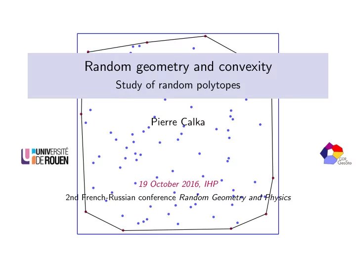
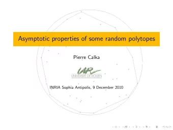
Random geometry and convexity Study of random polytopes Pierre - PowerPoint PPT Presentation

Random geometry and convexity Study of random polytopes Pierre Calka 19 October 2016, IHP 2nd French-Russian conference Random Geometry and Physics

default Point process Point process : random locally finite set of R d 1.0 1.0 1.0 0.9 0.9 0.9 0.8 0.8 0.8 0.7 0.7 0.7 0.6 0.6 0.6 0.5 0.5 0.5 0.4 0.4 0.4 0.3 0.3 0.3 0.2 0.2 0.2 0.1 0.1 0.1 0.0 0.0 0.0 0.0 0.1 0.2 0.3 0.4 0.5 0.6 0.7 0.8 0.9 1.0 0.0 0.1 0.2 0.3 0.4 0.5 0.6 0.7 0.8 0.9 1.0 0.0 0.1 0.2 0.3 0.4 0.5 0.6 0.7 0.8 0.9 1.0

default Point process without interaction �� �� �� �� �� �� �� �� �� �� �� �� �� �� �� �� �� �� � � � � �� �� B 4 B 1 �� �� � � �� �� �� �� �� �� �� �� � B 2 �� �� �� �� B 3 �� �� � �� �� �� �� �� �� � �� �� Binomial point process Poisson point process µ probability measure on R d µ σ -finite measure on R d X 1 , · · · , X n i.i.d. with law µ µ := intensity of the process E := { X 1 , · · · , X n } P locally finite set s.t. ◮ #( E ∩ B 1 ) binomial r.v. ( n , µ ( B 1 )) ◮ #( P ∩ B 1 ) Poisson r.v. ( µ ( B 1 )) ◮ #( E ∩ B 1 ) , · · · , #( E ∩ B ℓ ) not independent ◮ #( P ∩ B 1 ) , · · · , #( P ∩ B ℓ ) independent

default Uniform case Binomial model K := convex body of R d ( X k , k ∈ N ∗ ):= independent and uniformly distributed in K K n := Conv( X 1 , · · · , X n ), n ≥ 1 K 50 , K disk K 50 , K square

default Uniform case Binomial model K := convex body of R d ( X k , k ∈ N ∗ ):= independent and uniformly distributed in K K n := Conv( X 1 , · · · , X n ), n ≥ 1 K 100 , K disk K 100 , K square

default Uniform case Binomial model K := convex body of R d ( X k , k ∈ N ∗ ):= independent and uniformly distributed in K K n := Conv( X 1 , · · · , X n ), n ≥ 1 K 500 , K disk K 500 , K square

default Uniform case Poisson model K := convex body of R d P λ , λ > 0 := Poisson point process of intensity measure λ d x K λ := Conv( P λ ∩ K ) K 500 , K disk K 500 , K square

default Gaussian case Poisson model (2 π ) d / 2 e −� x � 2 / 2 , x ∈ R d , d ≥ 2 1 ϕ d ( x ) := P λ , λ > 0 := Poisson point process of intensity measure λϕ d ( x ) d x K λ := Conv( P λ ) K 100 K 500

default Plan Random polytopes: survey and new variance calculations Cases of the disk and the square: sketch of proof by scaling limit Poisson-Voronoi tessellation and isolated points Based on joint works with Joseph Yukich (Lehigh University, USA) and also Tomasz Schreiber (Toru´ n University, Poland), Yann Demichel & Nathana¨ el Enriquez (Paris Ouest)

default Plan Random polytopes: survey and new variance calculations Known expectation asymptotics Known second-order asymptotic results Main new results: exact limiting variances Cases of the disk and the square: sketch of proof by scaling limit Poisson-Voronoi tessellation and isolated points

default Known expectation asymptotics f k ( · ) := number of k -dimensional faces, Vol ( · ) := volume � 1 − E Vol ( K n − 1 ) � Efron’s relation (1965) E f 0 ( K n ) = n Vol ( K ) d − 1 1 Uniform, K smooth E [ f k ( K λ )] ∼ d s λ � d +1 d +1 c d , k ∂ K κ s λ →∞ κ s := Gaussian curvature of ∂ K d , k F ( K ) log d − 1 ( λ ) Uniform, K polytope E [ f k ( K λ )] ∼ c ′ λ →∞ F ( K ) := number of flags of K d − 1 2 ( λ ) Gaussian E [ f k ( K λ )] ∼ d , k log c ′′ λ →∞ A. R´ enyi & R. Sulanke (1963), H. Raynaud (1970), R. Schneider & J. Wieacker (1978), F. Affentranger & R. Schneider (1992)

default Known second-order asymptotic results ◮ Central limit theorems ◮ Variance bounds d − 1 d +1 ) Uniform, K smooth Var [ f k ( K λ )] λ →∞ Θ( λ = λ →∞ Θ(log d − 1 ( λ )) Uniform, K polytope Var [ f k ( K λ )] = d − 1 2 ( λ )) Gaussian Var [ f k ( K λ )] λ →∞ Θ(log = M. Reitzner (2005), I. B´ ar´ any & V. Vu (2007), I. B´ ar´ any & M. Reitzner (2010)

default Main new results: exact limiting variances d − 1 1 Uniform, K smooth Var [ f k ( K λ )] ∼ d s λ � d +1 c d , k ∂ K κ d +1 s λ →∞ κ s := Gaussian curvature of ∂ K d , k f 0 ( K ) log d − 1 ( λ ) Uniform, K simple polytope Var [ f k ( K λ )] ∼ c ′ λ →∞ d − 1 2 ( λ ) Gaussian Var [ f k ( K λ )] ∼ d , k log c ′′ λ →∞ Remarks ◮ Depoissonnization in the uniform smooth and Gaussian cases ◮ Central limit theorems ◮ Uniform in the ball and Gaussian cases: invariance principle for the volume

default Plan Random polytopes: survey and new variance calculations Cases of the disk and the square: sketch of proof by scaling limit Calculation of the variance of f k ( K λ ) Rescaling Floating body Dual characterization of extreme points Action of the scaling transform Convergence of the covariances of scores Poisson-Voronoi tessellation and isolated points

default Calculation of the expectation f k ( K λ ) Decomposition    � E [ f k ( K λ )] = E ξ ( x , P λ )  x ∈P λ 1 � k +1 # k -face containing x if x extreme ξ ( x , P λ ) := 0 if not Mecke-Slivnyak’s formula � E [ f k ( K λ )] = λ E [ ξ ( x , P λ ∪ { x } )] d x D

default Calculation of the variance of f k ( K λ ) Var [ f k ( K λ )]    � �  − ( E [ f k ( K λ )]) 2 ξ 2 ( x , P λ ) + = E ξ ( x , P λ ) ξ ( y , P λ ) x ∈P λ x � = y ∈P λ � E [ ξ 2 ( x , P λ ∪ { x } )] d x = λ D �� + λ 2 D 2 E [ ξ ( x , P λ ∪ { x , y } ) ξ ( y , P λ ∪ { x , y } )] d x d y �� − λ 2 D 2 E [ ξ ( x , P λ ∪ { x } )] E [ ξ ( y , P λ ∪ { y } )] d x d y � E [ ξ 2 ( x , P λ ∪ { x } )] d x = λ D �� + λ 2 D 2 Cov( ξ ( x , P λ ∪ { x } ) , ξ ( y , P λ ∪ { y } )) d x d y

default Rescaling Question Limits of E [ ξ ( x , P λ )] and Cov( ξ ( x , P λ ) , ξ ( y , P λ ))? Definition of limit scores in a new rescaled space Construction of the scaling transform Requires to understand the typical shape of K λ : the floating body.

default Floating body V ( x ) := inf { Vol ( K ∩ H + ) : H + half-plane containing x } , x ∈ K Floating body: K ( V ≥ t ) := { x ∈ K : V ( x ) ≥ t } K ( V ≥ t ) is a convex body and K ( V ≥ 1 /λ ) is close to K λ .

default Floating body V ( x ) := inf { Vol ( K ∩ H + ) : H + half-plane containing x } , x ∈ K Floating body : K ( V ≥ t ) := { x ∈ K : V ( x ) ≥ t } K ( V ≥ t ) is a convex body and K ( V ≥ 1 /λ ) is close to K λ . 1 D ( V ≥ 1 /λ ) = (1 − f ( λ )) D K ( V ≥ 1 /λ ) = { ( x 1 , x 2 ) : x 1 x 2 ≥ 2 λ } f ( λ ) ∼ c λ − 2 3

default Comparison between K λ and the floating body ◮ Expectation B´ ar´ any & Larman (1988): c Vol ( K ( V ≤ 1 /λ )) ≤ Vol ( K ) − E [ Vol ( K λ )] ≤ C Vol ( K ( V ≤ 1 /λ )) ◮ Variance any & Reitzner (2010): B´ ar´ c λ − 1 Vol ( K ( V ≤ 1 /λ )) ≤ Var [ Vol ( K λ )] ◮ Sandwiching B´ ar´ any & Reitzner (2010b): (log( λ )) − 16 � � P [ ∂ K λ �⊂ [ K ( V ≥ s ) \ K ( V ≥ T )]] = O λ (log( λ )) 17 , T := c ′ log(log( λ )) c s := λ

default Construction of the scaling transform Rules of the scaling transform ◮ One depth -coordinate provided by the family of floating 2 bodies: λ 3 (1 − r ) for the disk, λ x 1 x 2 for the quadrant ◮ One spatial -coordinate on the corresponding floating body ◮ A rescaling to guarantee Θ(1) points per unit area K = D � D \ { 0 } − → R × R + T λ : 1 2 ( r , θ ) �− → ( λ 3 θ, λ 3 (1 − r )) K = (0 , ∞ ) 2 � (0 , ∞ ) 2 − → L × R T ( λ ) : proj L (log( x )) , 1 � � ( x 1 , x 2 ) �− → 2 log( λ x 1 x 2 ) where L = { ( x 1 , x 2 ) ∈ R 2 : x 1 + x 2 = 0 }

default Dual characterization of extreme points Each point x generates a petal S ( x ), i.e. the set of all tangency points of curves K ( V = t λ ), t > 0, with the lines containing x . x is extreme if and only if its petal is not fully covered by the other petals. B d 0

default Action of the scaling transform in the disk Π ↑ := { ( v , h ) ∈ R × R + : h ≥ v 2 2 } , Π ↓ := { ( v , h ) ∈ R × R + : h ≤ − v 2 2 } Translate of Π ↓ Half-plane Boundary of the hull Union of portions of down-parabolas Translate of ∂ Π ↑ Petal ( x + Π ↑ ) not covered Extreme point Process P λ Process P of intensity d v d h Score ξ ( ∞ ) (( v , h ) , P ) Score ξ ( x , P λ ) B d − → 0

default Action of the scaling transform in the quadrant � � ch( v G ( v ) := log 2 ) , v ∈ V √ Π ↑ := { ( v , h ) ∈ R × R : h ≥ G ( v ) } , Π ↓ := { ( v , h ) ∈ R × R : h ≤ − G ( v ) } Floating bodies Horizontal half-planes Boundary of the hull Union of portions of pseudo-cones Translate of ∂ Π ↑ Petal ( x + Π ↑ ) not covered Extreme point √ 2 e 2 h d v d h Process P λ Process P of intensity Score ξ ( ∞ ) (( v , h ) , P ) Score ξ ( x , P λ ) − →