Random colored lattices Olivier Bernardi Joint work with Mireille - - PowerPoint PPT Presentation

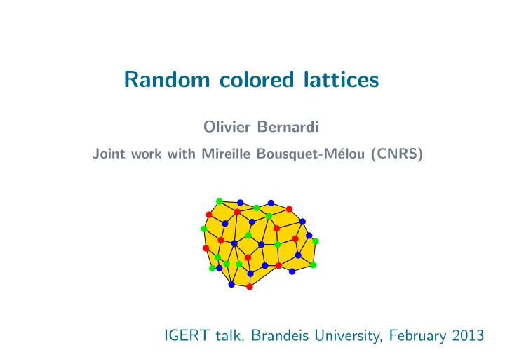
Random colored lattices

Olivier Bernardi

Joint work with Mireille Bousquet-M´ elou (CNRS)

IGERT talk, Brandeis University, February 2013

Random lattices, Random surfaces

A map is a way of gluing polygons in order to form a connected surface. Maps

A map is a way of gluing polygons in order to form a connected surface. Maps A planar map is a map on the sphere.

= =

A random lattice? Define a random lattice by choosing uniformly among all ways of gluing n = 1000 squares to form a planar map.

A random lattice? Define a random lattice by choosing uniformly among all ways of gluing n = 1000 squares to form a planar map. Theorem [Tutte 62] There are 2 · 3n (n + 1)(n + 2) 2n n

• rooted planar quadrangulations with n squares.

A random lattice? Define a random lattice by choosing uniformly among all ways of gluing n = 1000 squares to form a planar map. What kind of random object is it?

• A random graph.
• A random metric space: (V, d).

A random lattice? Define a random lattice by choosing uniformly among all ways of gluing n = 1000 squares to form a planar map. Properties of random lattices?

• What is the typical distance between two points?
• Are there small cycles separating two big pieces of the map?

A random lattice? Define a random lattice by choosing uniformly among all ways of gluing n = 1000 squares to form a planar map. Properties of random lattices?

• What is the typical distance between two points?

Theorem [Chassaing, Schaeffer 03] The distances scale as Cn n1/4, where Cn converges in law toward the law of the ”Integrated Super- Brownian Excursion” (up to a constant factor).

A random lattice? Define a random lattice by choosing uniformly among all ways of gluing n = 1000 squares to form a planar map. Properties of random lattices?

• What is the typical distance between two points?

Theorem [Chassaing, Schaeffer 03] The distances scale as Cn n1/4.

• Are there small cycles separating two big pieces of the map?

Theorem [LeGall 07, Miermont 09] No: if ǫ > 0 and f(n) → 0 then P(exists cycle of length < f(n) n1/4separating two pieces > ǫ n) → 0

How are such results proved?

• Bijection. [Cori Vauquelin 81, Schaeffer 98]

Rooted pointed quadrangulation with n faces. 2-to-1 Rooted plane trees with n edges +vertex labels changing by − 1, 0, 1 along edges and such that min=1. 2 2 1 1 1 3 3 2

How are such results proved?

• Bijection. [Cori Vauquelin 81, Schaeffer 98]

Rooted pointed quadrangulation with n faces. 2-to-1 Rooted plane trees with n edges +vertex labels changing by − 1, 0, 1 along edges and such that min=1. 3n · 1 (n + 1) 2n n

• 2

2 1 1 1 3 3 (n + 2) · 2 · 3n (n + 2)(n + 1) 2n n

• 2-to-1

2

How are such results proved?

• Bijection. [Cori Vauquelin 81, Schaeffer 98]

Rooted pointed quadrangulation with n faces. 2-to-1 Rooted plane trees with n edges +vertex labels changing by − 1, 0, 1 along edges and such that min=1.

Vertex at distance d from pointed vertex Vertex labeled d

2 2 1 1 1 3 3 2

How are such results proved?

• Bijection. [Cori Vauquelin 81, Schaeffer 98]

Rooted pointed quadrangulation with n faces. 2-to-1 Rooted plane trees with n edges +vertex labels changing by − 1, 0, 1 along edges and such that min=1.

Vertex at distance d from pointed vertex Vertex labeled d

2 2 1 1 1 3 3 2 2 1 1 3 3 2-to-1 2 2 2 1 1 1 3 3 2 1 2

Let Qn be the metric space (V,

d n1/4 ) corresponding to a uniformly

random quadrangulations with n faces. Random surfaces?

Let Qn be the metric space (V,

d n1/4 ) corresponding to a uniformly

random quadrangulations with n faces. Random surfaces? Theorem.[Le Gall 2007, Miermont/Le Gall 2012] The sequence Qn converges in distribution (in the Gromov Hausdorff topology) toward a random metric space, which

• is homeomorphic to the sphere
• has Hausdorff dimension 4.

distribution

Related work. Bouttier, Di Francesco, Chassaing, Guitter, Le Gall, Marckert, Miermont, Paulin, Schaeffer, Weill . . .

Random surfaces? The Brownian map is described in terms of

• Continuum Random Tree (= limit of discrete trees)
• Gaussian labels (= limit of discrete labels)

Brownian map 2 2 2 1 1 1 3 3 distribution Brownian map

Random surfaces? The Brownian map is described in terms of

• Continuum Random Tree (= limit of discrete trees)
• Gaussian labels (= limit of discrete labels)

Brownian map 2 2 2 1 1 1 3 3 distribution Brownian map

The Brownian map is universal: it is also the limit of uniformly random triangulations, etc.

Motivation: 2D quantum gravity. Right notion of random surface?

“There are methods and formulae in science, which serve as master-keys to many apparently different problems. The resources of such things have to be refilled from time to time. In my opinion at the present time we have to develop an art of handling sums over random surfaces. These sums replace the old-fashioned (and extremely useful) sums over random paths. The replacement is necessary, because today gauge invariance plays the central role in physics. Elementary excitations in gauge theories are formed by the flux lines (closed in the absence of charges) and the time develop- ment of these lines forms the world surfaces. All transition amplitudes are given by the sums over all possible surfaces with fixed boundary.” (A.M. Polyakov, Moscow, 1981.)

Motivation: 2D quantum gravity. Right notion of random surface? Two candidates for random surfaces:

• Discrete surfaces
• Brownian map
• Gaussian Free Field

“There are methods and formulae in science, which serve as master-keys to many apparently different problems. The resources of such things have to be refilled from time to time. In my opinion at the present time we have to develop an art of handling sums over random surfaces. These sums replace the old-fashioned (and extremely useful) sums over random paths. The replacement is necessary, because today gauge invariance plays the central role in physics. Elementary excitations in gauge theories are formed by the flux lines (closed in the absence of charges) and the time develop- ment of these lines forms the world surfaces. All transition amplitudes are given by the sums over all possible surfaces with fixed boundary.” (A.M. Polyakov, Moscow, 1981.)

Discrete version: Let h(x, y) be a function on {1, 2, . . . , n}2 chosen with probability density proportional to exp

• − 1

2

• e=(u,v)

(h(u) − h(v))2

• dh.

A glimpse at the Gaussian Free Field

Discrete version: Let h(x, y) be a function on {1, 2, . . . , n}2 chosen with probability density proportional to exp

• − 1

2

• e=(u,v)

(h(u) − h(v))2

• dh.

A glimpse at the Gaussian Free Field Use h to define a (random) ”density of area” on the square: Area(v) := exp(γh), and the (random) length of paths: Length(P) :=

• v∈P

exp(γh/2), where γ ∈ [0, 2).

Discrete version: Let h(x, y) be a function on {1, 2, . . . , n}2 chosen with probability density proportional to exp

• − 1

2

• e=(u,v)

(h(u) − h(v))2

• dh.

A glimpse at the Gaussian Free Field Continuous version: One would like to choose h on [0, 1]2 with a probability density proportional to exp

• − 1

2

• [0,1]2 ||∇h||2
• dh,

but does not make sense...

Discrete version: Let h(x, y) be a function on {1, 2, . . . , n}2 chosen with probability density proportional to exp

• − 1

2

• e=(u,v)

(h(u) − h(v))2

• dh.

A glimpse at the Gaussian Free Field Continuous version: One would like to choose h on [0, 1]2 with a probability density proportional to exp

• − 1

2

• [0,1]2 ||∇h||2
• dh,

but does not make sense... Solution: Take an orthonormal basis of functions {fi}i>0, and define h :=

i αifi with αi Gaussian.

The GFF h is not a function but a distribution: it is not defined at points, but the average in any region is well defined.

Question 1. Relation between Brownian map and Gaussian Free Field? Some big questions

Question 1. Relation between Brownian map and Gaussian Free Field? Some big questions Question 2. Parameter γ of GFF in terms of random maps?

Question 1. Relation between Brownian map and Gaussian Free Field? Some big questions Prediction from physics: The parameter γ of GFF is associated to the central charge c by γ = √25 − c − √1 − c √ 6 . and certain value of c can be achieved by adding a statistical mechanics model on the map. Example: No model is c = 0 and Ising model is c = 1/2. Question 2. Parameter γ of GFF in terms of random maps?

Idea: Instead of choosing a planar map of size n uniformly at random, let us choose it according to a statistical mechanics model. Maps chosen according to a statistical mechanics model. Example: Spanning-tree model. Choose maps with probability proportional to number of spanning trees.

Idea: Instead of choosing a planar map of size n uniformly at random, let us choose it according to a statistical mechanics model. Maps chosen according to a statistical mechanics model. Theorem [Mullin 67, Bernardi 07]. There are CatnCatn+1 rooted maps + spanning tree, where Catn =

1 n+1

2n

n

• .

Example: Spanning-tree model. Choose maps with probability proportional to number of spanning trees.

Maps chosen according to a statistical mechanics model.

• Question. Is the ”spanning-tree model” map really different ?

Maps chosen according to a statistical mechanics model.

• Question. Is the ”spanning-tree model” map really different ?

Simulation [Bernardi, Chapuy] The Hausdorff dimension of the spanning-tree model map is DH ≈ 3.5(5).

• Conj. [Watabiki 93]

DH = 2 √25 − c + √49 − c √25 − c + √1 − c ≈ 3.56 where c = −2 is central charge.

Maps chosen according to a statistical mechanics model.

• Question. Is the ”spanning-tree model” map really different ?

Easier information: asymptotic number of maps. Number of (rooted) maps with n edges is Mn ∼ k n−5/2 Rn. Number of maps+spanning trees: Tn ∼ k′ n−3 R′n

Maps chosen according to a statistical mechanics model.

• Question. Is the ”spanning-tree model” map really different ?

Easier information: asymptotic number of maps. Number of (rooted) maps with n edges is Mn ∼ k n−5/2 Rn. Theorem [Bender, Canfield 97+ Bernardi, Fusy 12] The exponent −5/2 is universal: same thing for any family of maps defined by face degree constraints + girth constraints. Number of maps+spanning trees: Tn ∼ k′ n−3 R′n The exponent is −3 also universal.

Maps chosen according to a statistical mechanics model.

• Question. Is the ”spanning-tree model” map really different ?

Easier information: asymptotic number of maps. Number of (rooted) maps with n edges is Mn ∼ k n−5/2 Rn. Number of maps+spanning trees: Tn ∼ k′ n−3 R′n Prediction from physics: α = 25 − c +

• (1 − c)(25 − c)

12 , where c is the central charge (c = 0 for maps without model, c = −2 for spanning-tree model).

Maps chosen according to a statistical mechanics model.

• Question. Is the ”spanning-tree model” map really different ?

Easier information: asymptotic number of maps. Number of (rooted) maps with n edges is Mn ∼ k n−5/2 Rn. Number of maps+spanning trees: Tn ∼ k′ n−3 R′n Prediction from physics: α = 25 − c +

• (1 − c)(25 − c)

12 , where c is the central charge (c = 0 for maps without model, c = −2 for spanning-tree model). KPZ formula [Knizhnik, Polyakov, Zamolodchikov 88]: Con- jecture relating critical exponents in regular lattices Vs random lattices.

Suppose number of objects of size n is Mn ∼ k n−αRn. Asymptotic number of maps and geometry?

s n − s

Sample a pair of objects of total size n. How small is the smallest one?

Suppose number of objects of size n is Mn ∼ k n−αRn. Asymptotic number of maps and geometry? Size of smallest one is s with probability proportional to ≈ k2 Rn (s(n − s))α . Thus, α big makes s n small.

s n − s

Sample a pair of objects of total size n. How small is the smallest one?

Potts model on maps

Potts model Configurations of the q-Potts model on a graph G are q-colorings. Their weight is ν#monochromatic edges. (parameters q, ν)

Potts model Configurations of the q-Potts model on a graph G are q-colorings. Their weight is ν#monochromatic edges. The partition function of the Potts model on the graph G is PG(q, ν) =

• q−coloring

ν#monochromatic edges. (parameters q, ν)

Potts model Configurations of the q-Potts model on a graph G are q-colorings. Their weight is ν#monochromatic edges. The partition function of the Potts model on the graph G is PG(q, ν) =

• q−coloring

ν#monochromatic edges. (parameters q, ν) Each coloring appears with probability ν#monochromatic edges PG(q, ν) .

Potts model PG(q, ν) =

• q−coloring

ν#monochromatic edges.

• The special case PG(q, 0) counts the proper q-colorings of G.
• The case q = 2 is the Ising model (without external field).

Potts model PG(q, ν) =

• q−coloring

ν#monochromatic edges.

• The special case PG(q, 0) counts the proper q-colorings of G.
• PG(q, ν) satisfies a recurrence relation:

PG(q, ν) = PG\e(q, ν) + (ν − 1) PG/e(q, ν).

deleted edge contracted edge

e G G\e G/e

• The case q = 2 is the Ising model (without external field).

Potts model PG(q, ν) =

• q−coloring

ν#monochromatic edges.

• The special case PG(q, 0) counts the proper q-colorings of G.
• PG(q, ν) is a polynomial in the variables q, ν

It is equivalent to the Tutte polynomial (a.k.a. partition function of the FK-Cluster model).

• PG(q, ν) satisfies a recurrence relation:

PG(q, ν) = PG\e(q, ν) + (ν − 1) PG/e(q, ν).

• The case q = 2 is the Ising model (without external field).

The Potts model on planar maps The partition function of the (annealed) Potts model on maps is G(q, ν, z) =

• M map

PM(q, ν)z#edges. This is a series in z with coefficients polynomial in q, ν.

The Potts model on planar maps The partition function of the (annealed) Potts model on maps is G(q, ν, z) =

• M map

PM(q, ν)z#edges. This is a series in z with coefficients polynomial in q, ν. Each map appears with probability PM(q, ν)z#edges G(q, ν, z)

The Potts model on planar maps The partition function of the (annealed) Potts model on maps is G(q, ν, z) =

• M map

PM(q, ν)z#edges. Goals:

• Characterize the partition function G(q, ν, z).

The Potts model on planar maps The partition function of the (annealed) Potts model on maps is G(q, ν, z) =

• M map

PM(q, ν)z#edges. Goals:

• Characterize the partition function G(q, ν, z).
• Study the phase transitions.

Example for q = 2 (Ising model): ν

zmax(ν) = radius of convergence of G(q, ν, z).

νc = (3 + √ 5)/2

The type of singularity of G(2, ν, z) is different at the critical value νc.

Method and results

Rooted plane trees with n edges: Warm up: Counting trees

n = 0 n = 1 n = 2 n = 3

Warm up: Counting trees Recursive decomposition:

+ =

Warm up: Counting trees Recursive decomposition:

+ =

We define the generating function: T(z) =

• T tree

z|T |. Decomposition gives T(z) = 1 +

• T1,T2 trees

z · z|T1| · z|T 2| = 1 + z T(z)2.

Warm up: Counting trees Recursive decomposition:

+ =

We define the generating function: T(z) =

• T tree

z|T |. T(z) = 1 + zT(z)2 ⇒ T(z) is algebraic: of the form Pol(T(z), z) = 0. ⇒ Number of trees with n edges ∼ k n−3/2 Rn. The exponent −3/2 is determined by the type of singularity of T(z).

Warm up: Counting trees Recursive decomposition:

+ =

We define the generating function: T(z) =

• T tree

z|T |. T(z) = 1 + zT(z)2 ⇒ T(z) is algebraic: of the form Pol(T(z), z) = 0. ⇒ Number of trees with n edges ∼ k n−3/2 Rn. Even better, using Lagrange inversion formula: ⇒ Number of trees with n edges Catn =

1 n+1

2n

n

• .

Method - comparative study

“Quadratic Method” M(1)=

• M map

z#edges Trees Maps (without Potts model)

= +

Generating function T =

• T tree

z#edges T = 1 + z T 2

= + +

Generating function M(x)=

• M map

xdeg0z#edges M(x) = 1 + x2zM(x)2 + xz xM(x)−M(1)

x−1

1−16z+(18z−1)M(1)−27z2M(1)2 = 0 algebraic equation algebraic equation functional equation with catalytic variable x

Method - comparative study

Maps with Potts model

+

functional equation with catalytic variables x, y [Tutte 71]

+

contracted edge deleted edge

Generating function G(x, y) ≡ G(x, y; q, ν, z)=

• M map

xdeg0 ydeg1 P(q, ν)z#edges G(x, y) = 1 + (q−1+u)x2yzG(x, y)G(x, 1) + uxy2zG(x, y)G(1, y) +

• xyz xG(x,y)−G(1,y)

x−1

− xyzG(x, y)G(1, y)

• +(u−1)
• xyz xG(x,y)−G(x,1)

y−1

− xyzG(x, y)G(x, 1)

• ?

Method Recursive decomposition of colored maps Functional equation for G(x, y; q, ν, z) with catalytic variables x, y. (a.k.a. loop equations) For q = 2 + 2 cos(kπ/m), functional equation for G(1, y; q, ν, z) Algebraic equations dependent on q Differential equation independent of q.

Generalization of “Quadratic Method” [Jehanne,Bousquet-M´ elou 06] Classical generatingfunctionology Method of invariants (core of our approach) Uniformization via some specializations y = Yi(z)

Method

Dm/2Tm

• N

2 √ D

• = m

r=0 Cr(z)Ir,

where D=(qν+(ν−1)2)I2−q(ν+1)I+z(q−4)(ν−1)(q+ν−1) + q, N=(4−q)(1/y−1)(ν−1)+(q+2ν−2)I − q I =yzqG(1, y)+ y−1

y

+

zy y−1

Algebraic equations dependent on q Differential equation independent of q.

Generalization of “Quadratic Method” Method of invariants (core of our approach) (for q = 2 + 2 cos(kπ/m)) Uniformization via some specializations y = Yi(z) functional equation with catalytic variables x, y G(x, y) = 1 + (q−1+u)x2yzG(x, y)G(x, 1) + uxy2zG(x, y)G(1, y) +

• xyz xG(x,y)−G(1,y)

x−1

− xyzG(x, y)G(1, y)

• +(u−1)
• xyz xG(x,y)−G(x,1)

y−1

− xyzG(x, y)G(x, 1)

• functional equation with catalytic variable y

Results about the Potts model on maps G(q, ν, z) =

• M map

PM(q, ν)z#edges. That is, for q =∈ {1, 2, 3, 2 + √ 2, 2 + √ 3, ...}, there is an equation of the form Polyq(G(q, ν, z), ν, z) = 0. Theorem [Bernardi, Bousquet-M´ elou]:

• The series G(q, ν, z) is algebraic whenever q = 2 + 2 cos(kπ/m)

and q = 0, 4.

Results about the Potts model on maps G(q, ν, z) =

• M map

PM(q, ν)z#edges. Theorem [Bernardi, Bousquet-M´ elou]:

• Some explicit algebraic equations for q = 2, 3.
• The series G(q, ν, z) is algebraic whenever q = 2 + 2 cos(kπ/m)

and q = 0, 4.

Results about the Potts model on maps G(q, ν, z) =

• M map

PM(q, ν)z#edges. Theorem [Bernardi, Bousquet-M´ elou]:

• Some explicit algebraic equations for q = 2, 3.

G(2, ν, z) = 1 + 3νS − 3νS2 − ν2S3 (1 − 2S + 2ν2S3 − ν2S4)2 ×

• ν3S6+2ν2(1−ν)S5+ν(1−6νS4−ν(1−5ν)S3+(1+2ν)S2−(3+ν)
• ,

where S = z + O(z2) is the series satisfying

S = z

• 1 + 3νS − 3νS2 − ν2S32

1 − 2S + 2ν2S3 − ν2S4 .

Example: For q = 2 (Ising model) we get:

• The series G(q, ν, z) is algebraic whenever q = 2 + 2 cos(kπ/m)

and q = 0, 4.

Results about the Potts model on maps G(q, ν, z) =

• M map

PM(q, ν)z#edges. Theorem [Bernardi, Bousquet-M´ elou]:

• Some explicit algebraic equations for q = 2, 3.
• The series G(q, ν, z) is algebraic whenever q = 2 + 2 cos(kπ/m)

and q = 0, 4. ν z zmax

νc = (3 + √ 5)/2

[zn]G(2, ν, z) ∼ cν n−5/2 Rn

ν if ν = νc,

[zn]G(2, ν, z) ∼ cν n−7/3 Rn

ν if ν = νc.

(matching the physicists’ predictions)

q = 2

= ⇒ Asymptotic results:

Results about the Potts model on maps G(q, ν, z) =

• M map

PM(q, ν)z#edges. Theorem [Bernardi, Bousquet-M´ elou]:

• There is a system of differential equations valid for all q.

Results about the Potts model on maps G(q, ν, z) =

• M map

PM(q, ν)z#edges. Theorem [Bernardi, Bousquet-M´ elou]:

There exists P(z, t)=

4

• i=0

Piti, Q(z, t)=

2

• i=0

Qiti, R(z, t)=

2

• i=0

Riti with Pi, Qi, Ri ∈ Q[q, ν][[z]] such that 1 Q ∂ ∂z Q2 P D2

• = 1

R ∂ ∂t R2 P D2

• .

with D = (qν + (ν − 1)2)t2 − q(ν + 1)t + z(q − 4)(ν − 1)(q + ν − 1) + q and P4 = 1, R2 = 3 − ν − q, P(0, t) = t2(t − 1)2, Q(0, t) = t(t − 1). These series are unique and determine G(q, ν, z) through: 12 z2(qν + (ν − 1)2)G(q, ν, z) = P2 − 2 Q0 − 8 z(3 − ν − q)Q1 − Q2

1 + 4 z(3 ν − 2 + q) − 12 z2(3 − ν − q)2.

• There is a system of differential equations valid for all q.

Results about the Potts model on Triangulations G(q, ν, z) =

• M triangulation

PM(q, ν)z#edges. Theorem [Bernardi, Bousquet-M´ elou]:

• Some explicit algebraic equations for q = 2, 3.
• There is a system of differential equations valid for all q.
• The series G(q, ν, z) is algebraic whenever q = 2 + 2 cos(kπ/m)

and q = 0, 4.

Other results: For planar maps, [Guionnet, Jones, Shlyakhtenko, Zinn-Justin 2012] give a functional equation for G(q, ν, z) in terms of Theta functions.

Other results:

Denote α and β the weight of monochromatic and dichromatic edges and denote δ = q2 = 2cos(σπ) with σ ∈ R, and denote C(δ, α, β) = G(q, ν, z). Then the series C(γ; δ, α, β) with “catalytic variable” γ is given in terms of a series M(γ) by: C(γ; δ, α, β) = h(γ)α γ M(h(γ)), where h(γ) is the inverse of the function g(z) = zα 1−z2M(z) Moreover, M(γ) and four auxiliary series a1 < a2 < b1 < b2 in δ, α, β are simultaneously defined by: 1 z(u) M

• α

z(u)

• =

1 q + q−1  ϕ(u) + ϕ(−u) + 2q z(u) (1 − q2)α + (q2 + 1)(z(u) − 1) (1 − q2)β   , where ϕ(u) = c+ Θ(u − u∞ − 2σK) Θ(u − u∞) + c− Θ(u + u∞ − 2σK) Θ(u + u∞) , and z(u) is the functional inverse of u(z) = i 2

• (b1 − a1)(b2 − a2)

z b2 dx

• (x − a1)(x − a2)(x − b1)(x − b2)

, and Θ(u) denotes a Theta function with periods K, K′, and K, K′, u∞, z∞, c± are constant given in terms

• f a1, b1, α, β, δ.

For planar maps, [Guionnet, Jones, Shlyakhtenko, Zinn-Justin 2012] give a functional equation for G(q, ν, z) in terms of Theta functions.

Other results: For planar maps, [Guionnet, Jones, Shlyakhtenko, Zinn-Justin 2012] give a functional equation for G(q, ν, z) in terms of Theta functions. [Bonnet, Eynard 99] give similar results for triangulations.

Other results: For planar maps, [Guionnet, Jones, Shlyakhtenko, Zinn-Justin 2012] give a functional equation for G(q, ν, z) in terms of Theta functions. [Bonnet, Eynard 99] give similar results for triangulations. For properly colored triangulations [Tutte 73-84] gives a differential equation for H = G(q, 0, z): 2q2(1−q)z+(qz+10H−6zH′)H′′+q(4−q)(20H−18zH′+9z2H′′)=0.

Other results: For planar maps, [Guionnet, Jones, Shlyakhtenko, Zinn-Justin 2012] give a functional equation for G(q, ν, z) in terms of Theta functions. [Bonnet, Eynard 99] give similar results for triangulations. This is our guide, but the proof is long!

[Tutte 73] Chromatic sums for rooted planar triangulations: the cases λ=1 and λ=2. [Tutte 73] Chromatic sums for rooted planar triangulations, II: the case λ = τ + 1. [Tutte 73] Chromatic sums for rooted planar triangulations, III: the case λ = 3. [Tutte 73] Chromatic sums for rooted planar triangulations, IV: the case λ = ∞. [Tutte 74] Chromatic sums for rooted planar triangulations, V: special equations. [Tutte 78] On a pair of functional equations of combinatorial interest. [Tutte 82] Chromatic solutions. [Tutte 82] Chromatic solutions II. [Tutte 84] Map-colourings and differential equations. Summarized in: [Tutte 95] Chromatic sums revisited.

For properly colored triangulations [Tutte 73-84] gives a differential equation for H = G(q, 0, z): 2q2(1−q)z+(qz+10H−6zH′)H′′+q(4−q)(20H−18zH′+9z2H′′)=0.

Open questions Question 1. Can we translate the system of differential equations to just one differential equation?

Open questions Question 1. Can we translate the system of differential equations to just one differential equation? Question 2. Can we obtain asymptotic growth of coefficients for the

• ther values of q?

Open questions Question 1. Can we translate the system of differential equations to just one differential equation? Question 2. Can we obtain asymptotic growth of coefficients for the

• ther values of q?

Question 3. Generating function is algebraic for q = 2 + 2 cos(kπ/m). Is there a bijection with trees for these values of q? Theorem [Bernardi, Fusy 12] For maps without matter, any family defined by degree of faces + girth constraints has an algebraic gen- erating function, and is in bijection with a family of trees (defined by local degree constraints).

Thanks.