Quiz Parts 1 and 2: Describe two interpretations of the matrix-vector - PowerPoint PPT Presentation

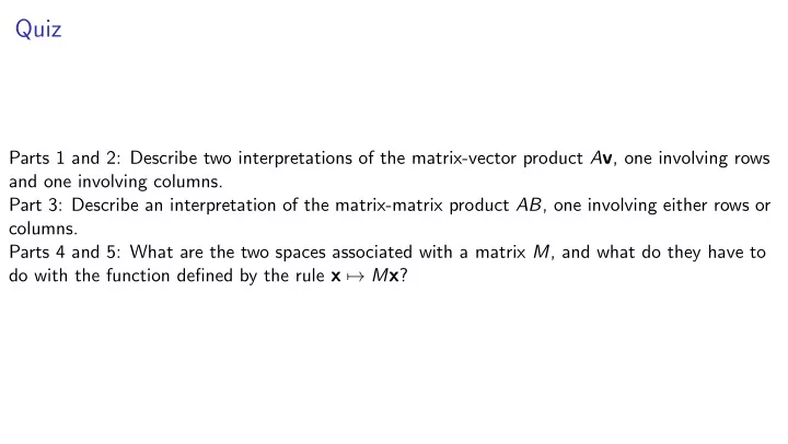
Quiz Parts 1 and 2: Describe two interpretations of the matrix-vector product A v , one involving rows and one involving columns. Part 3: Describe an interpretation of the matrix-matrix product AB , one involving either rows or columns. Parts 4 and 5: What are the two spaces associated with a matrix M , and what do they have to do with the function defined by the rule x 7! M x ?

Matrix-vector equation for sensor node Define D = { ’radio’, ’sensor’, ’memory’, ’CPU’ } . Goal: Compute a D -vector u that, for each hardware component, gives the current drawn by that component. Four test periods: I total milliampere-seconds in these test periods b = [140 , 170 , 60 , 170] I for each test period, vector specifying how long each hardware device was operating: I duration 1 = Vec(D, ’radio’:.1, ’CPU’:.3) I duration 2 = Vec(D, ’sensor’:.2, ’CPU’:.4) I duration 3 = Vec(D, ’memory’:.3, ’CPU’:.1) I duration 4 = Vec(D, ’memory’:.5, ’CPU’:.4) 2 duration 1 3 duration 2 6 7 To get u , solve A ⇤ x = b where A = 6 7 duration 3 4 5 duration 4

The solver module, and floating-point arithmetic For arithmetic over R , Python uses floats, so round-o ff errors occur: >>> 10.0**16 + 1 == 10.0**16 True Consequently algorithms such as that used in solve(A, b) do not find exactly correct solutions. To see if solution u obtained is a reasonable solution to A ⇤ x = b , see if the vector b � A ⇤ u has entries that are close to zero: >>> A = listlist2mat([[1,3],[5,7]]) >>> u = solve(A, b) >>> b - A*u Vec({0, 1},{0: -4.440892098500626e-16, 1: -8.881784197001252e-16}) The vector b � A ⇤ u is called the residual . Easy way to test if entries of the residual are close to zero: compute the dot-product of the residual with itself: >>> res = b - A*u >>> res * res 9.860761315262648e-31

Checking the output from solve(A, b) For some matrix-vector equations A ⇤ x = b , there is no solution. In this case, the vector returned by solve(A, b) gives rise to a largeish residual: >>> A = listlist2mat([[1,2],[4,5],[-6,1]]) >>> b = list2vec([1,1,1]) >>> u = solve(A, b) >>> res = b - A*u >>> res * res 0.24287856071964012 Some matrix-vector equations are ill-conditioned , which can prevent an algorithm using floats from getting even approximate solutions, even when solutions exists: >>> A = listlist2mat([[1e20,1],[1,0]]) We will not study conditioning in >>> b = list2vec([1,1]) >>> u = solve(A, b) this course. >>> b - A*u Vec({0, 1},{0: 0.0, 1: 1.0})

Triangular matrix We can rewrite this linear system as a Recall: We considered triangular linear matrix-vector equation: systems, e.g. ] · x [ 1 , 0 . 5 , � 2 , 4 = � 8 2 1 0 . 5 � 2 4 3 [ 0 , 3 , 3 , 2 ] · x = 3 0 3 3 2 6 7 5 ⇤ x = [ � 8 , 3 , � 4 , 6] ] · x [ 0 , 0 , 1 , 5 = � 4 6 7 0 0 1 5 4 [ 0 , 0 , 0 , 2 ] · x = 6 0 0 0 2 [ 0 , 0 , 0 , 2 ] · x = 6 The matrix is a triangular matrix. Definition: An n ⇥ n upper triangular matrix A is a matrix with the property that A ij = 0 for i > j . Note that the entries forming the upper triangle can be be zero or nonzero. We can use backward substitution to solve such a matrix-vector equation. Triangular matrices will play an important role later.

Algebraic properties of matrix-vector multiplication Proposition: Let A be an R ⇥ C matrix. I For any C -vector v and any scalar α , A ⇤ ( α v ) = α ( A ⇤ v ) I For any C -vectors u and v , A ⇤ ( u + v ) = A ⇤ u + A ⇤ v

Algebraic properties of matrix-vector multiplication To prove A ⇤ ( α v ) = α ( A ⇤ v ) we need to show corresponding entries are equal: Need to show entry i of A ⇤ ( α v ) = entry i of α ( A ⇤ v ) 2 3 a 1 . . Proof: Write A = 5 . 6 7 . 4 a m By dot-product def. of matrix-vector mult, By definition of scalar-vector multiply, entry i of A ⇤ ( α v ) = a i · α v entry i of α ( A ⇤ v ) = α (entry i of A ⇤ v ) = α ( a i · v ) = α ( a i · v ) by homogeneity of dot-product by dot-product definition of matrix-vector multiply QED

Algebraic properties of matrix-vector multiplication To prove A ⇤ ( u + v ) = A ⇤ u + A ⇤ v we need to show corresponding entries are equal: Need to show entry i of A ⇤ ( u + v ) = entry i of A ⇤ u + A ⇤ v 2 3 a 1 . . Proof: Write A = 5 . 6 7 . 4 a m By dot-product def. of matrix-vector mult, By dot-product def. of matrix-vector mult, entry i of A ⇤ ( u + v ) = a i · ( u + v ) entry i of A ⇤ u = a i · u = a i · u + a i · v entry i of A ⇤ v = a i · v so by distributive property of dot-product entry i of A ⇤ u + A ⇤ v = a i · u + a i · v QED

Matrix-matrix multiplication and function composition Corresponding to an R ⇥ C matrix A over a field F , there is a function f : F C � ! F R namely the function defined by f ( y ) = A ⇤ y

Matrix-matrix multiplication and function composition Matrices A and B ) functions f ( y ) = A ⇤ y and g ( x ) = B ⇤ x and h ( x ) = ( AB ) ⇤ x Matrix-Multiplication Lemma f � g = h Example:  1 ✓ x 1  1 �  x 1  x 1 + x 2 � �◆ � � 1 1 A = ) f = = 0 1 x 2 0 1 x 2 x 2  1 ✓ x 1  1 �  x 1 0 � �◆ 0 �  � x 1 B = = = ) g 1 1 x 2 1 1 x 2 x 1 + x 2  1 �  1  2 1 0 � 1 � product AB = = 0 1 1 1 1 1 ✓ x 1  2 �  x 1  2 x 1 + x 2 �◆ � � 1 corresponds to function h = = 1 1 x 1 + x 2 x 2 x 2 ✓ x 1  2 x 1 + x 2 �◆ ✓ �◆ � x 1 = f = so f � g = h f � g x 1 + x 2 x 1 + x 2 x 2

Matrix-matrix multiplication and function composition Matrices A and B ) functions f ( y ) = A ⇤ y and g ( x ) = B ⇤ x and h ( x ) = ( AB ) ⇤ x Matrix-Multiplication Lemma: f � g = h Proof: Let columns of B be b 1 , . . . , b n . By the matrix-vector definition of matrix-matrix multiplication, column j of AB is A ⇤ (column j of B ). For any n -vector x = [ x 1 , . . . , x n ], g ( x ) = B ⇤ x by definition of g = x 1 b 1 + · · · + x n b n by linear combinations definition Therefore f ( g ( x )) = f ( x 1 b 1 + · · · x n b n ) = x 1 ( f ( b 1 )) + · · · + x n ( f ( b n )) by algebraic properties = x 1 ( A ⇤ b 1 ) + · · · + x n ( A ⇤ b n ) by definition of f = x 1 (column 1 of AB ) + · · · + x n (column n of AB ) by matrix-vector def. = ( AB ) ⇤ x by linear-combinations def. = h ( x ) by definition of h

Associativity of matrix-matrix multiplication Matrices A and B ) functions f ( y ) = A ⇤ y and g ( x ) = B ⇤ x and h ( x ) = ( AB ) ⇤ x Matrix-Multiplication Lemma: f � g = h Matrix-matrix multiplication corresponds to function composition. Corollary: Matrix-matrix multiplication is associative: ( AB ) C = A ( BC ) Proof: Function composition is associative. QED Example:  1 � ✓ 1  1 �  0  0 �  � 1 �◆ � � 0 1 3 0 5 5 = = 1 1 0 1 1 2 1 1 1 2 1 7 ✓ 1 �  1  1  0 �◆  � 1 �  � 1 � � � 0 1 3 1 3 5 = = 1 1 0 1 1 2 1 2 1 2 1 7

Matrices and their functions Now we study the relationship between a matrix M and the function x 7! M ⇤ x I Easy: Going from a matrix M to the function x 7! M ⇤ x I A little harder: Going from the function x 7! M ⇤ x to the matrix M . In studying this relationship, we come up with the fundamental notion of a linear transformation .

From matrix to function Starting with a M , define the function f ( x ) = M ⇤ x . Domain and co-domain? If M is an R ⇥ C matrix over F then I domain of f is F C I co-domain of f is F R # @ ? Example: Let M be the matrix and define f ( x ) = M ⇤ x a 1 2 3 10 20 30 b I Domain of f is R { # , @ , ? } . # @ ? a b f maps to 2 2 -2 0 0 I Co-domain of f is R { a , b } .  1 � 2 3 Example: Define f ( x ) = ⇤ x . 10 20 30 I Domain of f is R 3 f maps [2 , 2 , � 2] to [0 , 0] I Co-domain of f is R 2

From function to matrix We have a function f : F A � ! F B We want to compute matrix M such that f ( x ) = M ⇤ x . I Since the domain is F A , we know that the input x is an A -vector. I For the product M ⇤ x to be legal, we need the column-label set of M to be A . I Since the co-domain is F B , we know that the output f ( x ) = M ⇤ x is B -vector. I To achieve that, we need row-label set of M to be B . Now we know that M must be a B ⇥ A matrix.... ... but what about its entries?

From function to matrix I We have a function f : F n � ! F m I We think there is an m ⇥ n matrix M such that f ( x ) = M ⇤ x How to go from the function f to the entries of M ? 2 3 4 v 1 I Write mystery matrix in terms of its columns: M = · · · v n 5 I Use standard generators e 1 = [1 , 0 , . . . , 0 , 0] , . . . , e n = [0 , . . . , 0 , 1] with linear-combinations definition of matrix-vector multiplication: 2 3 4 v 1 5 ⇤ [1 , 0 , . . . , 0 , 0] = v 1 f ( e 1 ) = · · · v n . . . 2 3 4 v 1 5 ⇤ [0 , 0 , . . . , 0 , 1] = v n f ( e n ) = · · · v n

From function to matrix: horizontal scaling Define s ([ x , y ]) = stretching by two in horizontal direction Assume s ([ x , y ]) = M ⇤ [ x , y ] for some matrix M . I We know s ([1 , 0]) = [2 , 0] because we are stretching by two in horizontal direction I We know s ([0 , 1]) = [0 , 1] because no change in vertical direction.  2 � 0 Therefore M = 0 1