Quantum Violation of Fluctuation-Dissipation Theorem Akira Shimizu - PowerPoint PPT Presentation
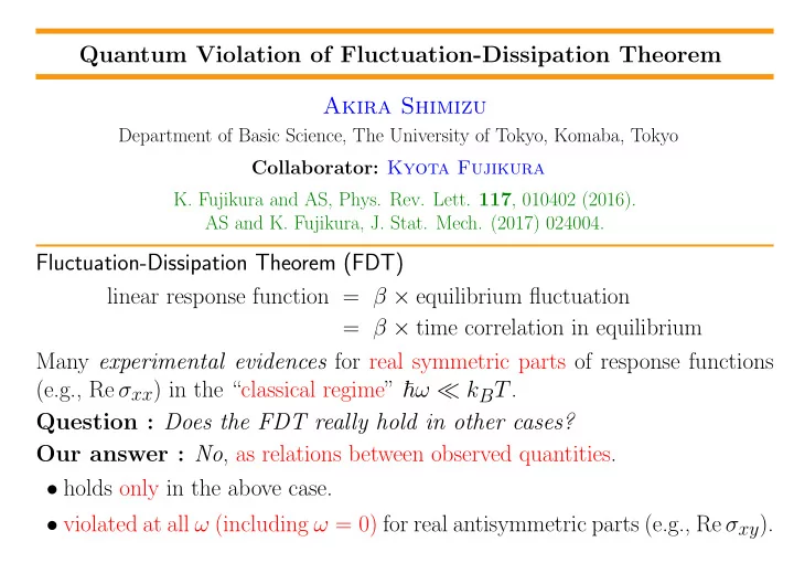
Quantum Violation of Fluctuation-Dissipation Theorem Akira Shimizu Department of Basic Science, The University of Tokyo, Komaba, Tokyo Collaborator: Kyota Fujikura K. Fujikura and AS, Phys. Rev. Lett. 117 , 010402 (2016). AS and K. Fujikura, J.
Quantum Violation of Fluctuation-Dissipation Theorem Akira Shimizu Department of Basic Science, The University of Tokyo, Komaba, Tokyo Collaborator: Kyota Fujikura K. Fujikura and AS, Phys. Rev. Lett. 117 , 010402 (2016). AS and K. Fujikura, J. Stat. Mech. (2017) 024004. Fluctuation-Dissipation Theorem (FDT) linear response function = β × equilibrium fluctuation = β × time correlation in equilibrium Many experimental evidences for real symmetric parts of response functions (e.g., Re σ xx ) in the “classical regime” � ω ≪ k B T . Question : Does the FDT really hold in other cases? Our answer : No , as relations between observed quantities. • holds only in the above case. • violated at all ω (including ω = 0) for real antisymmetric parts (e.g., Re σ xy ).
Motivation Nothing moves in Gibbs states. In the thermal pure quantum states, macrovariables do not move, whereas mi- crovariables move. To calculate fluctuation of macrovariables, we must calculate time correlation. But, when we look at an equilibrium state, macrovariables do move (fluctuate). ✓ ✏ My question: What is the quantum state in which macrovariables fluctuate? ✒ ✑ Kyota Fujikura (M1 at that time) got interested in this question. ⇒ He constructed a ‘squeezed equilibrium state’ (shown later). Such a state should be found, e.g., just after measurement. ✓ ✏ My question: Is it a universal result? ✒ ✑ He answered yes. ⇒ I was upset because I realized it implies universal violation of FDT! ⇒ Detailed analysis.
Contents 1. What’s wrong with derivations of the FDT? 2. Assumptions (a) on the system and its equilibrium states (b) on measurements 3. Measurement of time correlation 4. Violation of FDT 5. Experiments on violation 6. Discussions 7. Summary 8. Additional comments (if time allows)
What’s wrong with derivations of the FDT? H. Takahashi (J. Phys. Soc. Jpn. 7, 439 (1952)) • derived the FDT for classical systems. • About its translation to quantum systems: “profound difficulty that every observation disturbs the system.” � B ( t ) � B ( t ) F ( t ) time time F ( t )=0 measurement of response measurement of fluctuation տ ր disturbances by quantum measurements
What’s wrong with derivations of the FDT? (continnued) Callen and Welton (1951) and Kubo (1957) • “Derived” the FDT for quantum systems from the Schr¨ odinger equation. • Neglected the disturbances by measurements. Nevertheless, ‘Kubo formula’ is often regarded as a proof of the FDT. ✓ ✏ Kubo : linear response function = β × canonical time correlation* disturbance → � ? disturbance → � ? FDT : linear response function = β × time correlation in equilibrium observed one observed one ✒ ✑ * canonical time correlation: � β Y ( t ) � eq ≡ 1 � e λ ˆ Xe − λ ˆ H ˆ H ˆ � ˆ X ; ˆ Y ( t ) � eq dλ β 0
What’s wrong with derivations of the FDT? (continnued) Question: Are macrovariables so affected by quantum disturbance? Our answer: • No, when response is measured. ⇒ Kubo formula may be correct as a recipe to obtain response functions. • Yes, when fluctuarion is measured. ⇒ canonical time correlation � = observed time correlation. ✓ ✏ Kubo : linear response function = β × canonical time correlation disturbance → / � disturbance → ∦ ∦ ∦ FDT : linear response function � = β × time correlation in equilibrium observed one observed one ✒ ✑ FDT is violated as relations between observed quantities.
Contents 1. What’s wrong with derivations of the FDT? 2. Assumptions (a) on the system and its equilibrium states (b) on measurements 3. Measurement of time correlation 4. Violation of FDT 5. Experiments on violation 6. Discussions 7. Summary 8. Additional comments (if time allows)
Assumptions on the system and its equilibrium states d -dimensional macroscopic system ( d = 1 , 2 , 3 , · · · ) of size N (e.g., # of spins) • Equilibrium state of temperature T (= 1 /β ) thermal pure quantum state | β � (same results as the Gibbs state) S. Sugiura ans AS, PRL 108 , 240401 (2012); PRL 111 , 010401 (2013). � · � eq = � β | · | β � • Assumption Correlation between local observables decays faster than 1 /r d + ǫ ( ǫ > 0). ♣ holds generally, except at citical points. ⇒ For all additive observable ˆ A (= � r same local observable), √ � � (∆ ˆ A ) 2 � eq = O ( δA eq ≡ N ) . ∆ ˆ A ≡ ˆ A − � ˆ A � eq ; throughout this talk ∆ denotes deviation from the equilibrium value. • Additional reasonable assumptions ⇒ Q uantum C entral L imit T heorem (D. Goderis and P. Vets (1989); T. Matsui (2002).) ♣ We do not write N ∝ V →∞ explicitly, except when we want to stress it. lim
Contents 1. What’s wrong with derivations of the FDT? 2. Assumptions (a) on the system and its equilibrium states (b) on measurements 3. Measurement of time correlation 4. Violation of FDT 5. Experiments on violation 6. Discussions 7. Summary 8. Additional comments (if time allows)
Assumptions on measurements If a violent detector, ⇒ completely destroys the state by the 1st measurement ⇒ meaningless result for the 2nd measurement ⇒ wrong result for the correlation To measure the time correlation correctly, “ideal” detectors should be used. Classical systems ideal detector ≡ a detector that does not disturb the state at all. Quantum systems Such a detector is impossible! ⇒ Use a detector that simulates the classical ideal one as closely as possible. “quasiclassical measurement” To examine the validity of the FDT in quantum systems, we must assume quasiclassical measurements.
Assumptions on measurements (continued) quasiclassical measurement should have a moderate magnitude of error: • δA err < δA eq . • δA err ց ⇒ disturbance ր ⇒ δA err should not be too small. We require δA err = εδA eq ( ε : a small positive onstant) . ♣ Our results hold also for larger ε . √ Since δA eq = O ( N ), √ δA err = O ( N ) . To formulate measurements of equilibrium fluctuations, use √ a = ˆ A/ N ˆ ⇒ δa eq = O (1) , δa err = O (1) .
Assumptions on measurements (continued) General framework of quantum measurement (adapted to our problem) Pre-measurement state = | ψ � (uniform macroscopically) Measurement of an additive observable ˆ A → outcome A • (real valued variable) ♣ δA err > 0 ⇒ A • is not necessarily one of eigenvalues. √ ♣ a • ≡ A • / N can be regarded as a continuous variable. Probability density of getting a • : p ( a • ) = � ψ | ˆ E a • | ψ � E a • : probability operator (Hermitian, positive semidefinite, integral = ˆ ˆ 1) ˆ E a • can be decomposed as M † E a • = ˆ ˆ a • ˆ M a • M a • : measurement operator (not unique for a given ˆ ˆ E a • ) 1 ˆ Post-measurement state = M a • | ψ � � p ( a • )
Assumptions on measurements (continued) M † p ( a • ) = � ψ | ˆ E a • = ˆ ˆ a • ˆ a • : outcome , E a • | ψ � , M a • Definiton: quasiclassical measurement of additive observables ✓ ✏ (i) unbiased : a • = � ˆ a � eq ( · · · = average over many runs of experiments) ∵ Otherwise, the FDT would look more violated. (ii) For | β � , p shifted (∆ a • ) ≡ p ( a • ) converges as N → ∞ . ⇒ e.g., measurement error δA err = εδA eq , as required. M † N † (iii) ˆ M a • is minimally disturbing among ˆ E a • = ˆ a • ˆ M a • = ˆ a • ˆ N a • = · · · . � ˆ ˆ ⇒ M a • = E a • (iv) homogeneous , i.e., ˆ E a • depends on ˆ a and a • only through ˆ a − a • . ⇒ e.g., δa err = independent of a • . ˆ From (i)-(iv), M a • = f (ˆ a − a • ), where f ( x ) ≥ 0. (v) f ( x ) behaves well enough . e.g., it vanishes quickly as | x | → ∞ (see paper for details) ✒ ✑
Assumptions on measurements (continued) Roughly speaking, quasiclassical measeurment is • unbiased • homogeneous • minimally-disturbing • moderate magnitudes of error (small enough to measure fluctuations, but not too small in order to avoid strong disturbances.) ex. Gaussian measurement operator ✓ ✏ � � − x 2 1 f ( x ) = (2 πw 2 ) 1 / 4 exp , w = O (1) > 0 . 4 w 2 ✒ ✑ � � a − a • ) 2 1 − (ˆ ˆ M a • = f (ˆ a − a • ) = (2 πw 2 ) 1 / 4 exp , 4 w 2 √ √ δa err = w = O (1) ( δA err = w N = O ( N )) .
Contents 1. What’s wrong with derivations of the FDT? 2. Assumptions (a) on the system and its equilibrium states (b) on measurements 3. Measurement of time correlation 4. Violation of FDT 5. Experiments on violation 6. Discussions 7. Summary 8. Additional comments (if time allows)
Measurement of time correlation ✓ ✏ t = 0 − : equilibrium state = | β � (thermal pure quantum state) ↓ √ √ t = 0 : measurement of ˆ A = ˆ a N ⇒ outcome A • = a • N 1 post-measurement state = | β ; a • � = f (ˆ a − a • ) | β � � p ( a • ) ↓ free evolution t > 0 : e − i ˆ Ht/ � | β ; a • � measurement of ˆ A (or another additive operator ˆ B ) ⇒ outcome ⇓ From the two outcomes .... Obtain : correlation of ˆ A (0) and ˆ A ( t ) (or ˆ B ( t )) ✒ ✑ • 1st measurement should be quasiclassical (to minimize disturbance) • 2nd measurement can be either quasiclassical or error-less. (Because its post-measurement state will not be measured.)
Recommend
More recommend
Explore More Topics
Stay informed with curated content and fresh updates.
