Quantum Tunneling and Decoherence in Coherently Driven Double-Well - PDF document

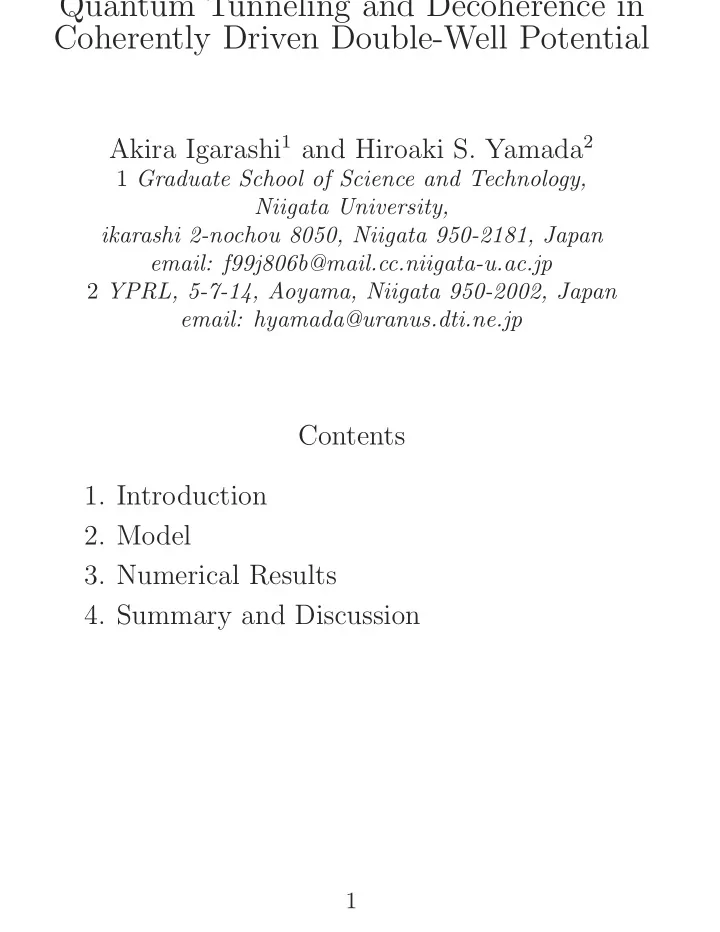
Quantum Tunneling and Decoherence in Coherently Driven Double-Well Potential Akira Igarashi 1 and Hiroaki S. Yamada 2 1 Graduate School of Science and Technology, Niigata University, ikarashi 2-nochou 8050, Niigata 950-2181, Japan email: f99j806b@mail.cc.niigata-u.ac.jp 2 YPRL, 5-7-14, Aoyama, Niigata 950-2002, Japan email: hyamada@uranus.dti.ne.jp Contents 1. Introduction 2. Model 3. Numerical Results 4. Summary and Discussion 1

1 Introduction We numerically investigate influence of a polychromatic perturbation on wave packet dynamics in one-dimensional double-well potential. Some interesting results are known in monochromatic perturbed double-well system, such as enhancement or suppression of tunneling between the wells, however tunneling dynamics in polychromatically perturbed double well does not seem to be clear. In order to make it clear, we consider tunneling dynamics the one-dimensional double-well driven by coherent external field. Especially we consider the following problem. • Does coherent tunneling occur under the perturba- tion ? • Does one remain against strong perturbation ? • If the coherence of the tunneling dynamics is de- stroyed, what kind of motion becomes dominant ? 2

2 Model The model system is coherently driven one-dimensional double-well whose Hamiltonian is, H ( p, q, t ) = p 2 2 + q 4 4 − A ( t ) q 2 (1) 2 , M 1 � A ( t ) = a − √ ǫ i sin(Ω i t + θ i ) . (2) M j =1 Here A ( t ) describes time-dependent perturbation and, • q, p : Canonically conjugate position and momentum. • a : The parameter determining the distance between the potential well. • M : The number of frequency component. • { ǫ i } : The i ’s perturbation strength. • { Ω i } : Mutually incommensurate and oder of unity frequencies of the external perturbation. • { θ i } : The initial phases of the external driving force. To make some energy doublets and for simplicity we set a = 5, ǫ i = ǫ = 0 . 1 ∼ 1 . 0, and θ i ’s are random numbers. We take off-resonant frequencies which are far from resonance in the corresponding unperturbed problem in order to avoid energy absorption due to resonance. 3

Time dependence of the potential, the initial wave packet, and some lowest unperturbed eigen energy levels are shown Fig. 1. 8 t= 0 t= π / 2 Ω 1 6 t= 3 π / 2 Ω 1 4 2 V ( q,t ) 0 -2 -4 -6 -8 -3 -2 -1 0 1 2 3 q Fig. 1: The sketch of the potential at some mo- ments, the initial packet and some eigen energy. The classical phase space structure of this system are shown below. (a) M= 1 , � = 0 . 1 (b) M= 2 , � = 0 . 1 0.8 0.8 0.6 0.6 0.4 0.4 p 0.2 p 0.2 0 0 -0.2 -0.2 -0.4 -0.4 -0.6 -0.6 -0.8 -0.8 -1 -1 -1 -1 1.9 2 2.1 2.2 2.3 2.4 2.5 2.6 1.9 2 2.1 2.2 2.3 2.4 2.5 2.6 q q (c) M= 10 , � = 0 . 6 (d) M= 10 , � = 1 . 0 8 5 6 4 3 4 2 2 1 p p 0 0 -1 -2 -2 -4 -3 -6 -4 -5 -8 -4 -3 -2 -1 0 1 2 3 4 -4 -3 -2 -1 0 1 2 3 4 q q Fig. 2: Points are plotted at t = 2 πn/ Ω 1 in each cases. 4

3 Numerical Results 3.1 Tunneling To calculate wave packet tunneling, we use the following Gaussian localized as the initial state, which is localized in the right well of the potential, ψ ( q, t = 0) = exp {− ( q − q 0 ) 2 } . (3) 2 σ • q 0 : the right bottom of the potential well. • σ : the initial spread of the packet. We set σ = 0 . 3. This initial packet approximates equal- weight linear combination of the unperturbed lowest dou- blet. We then define P L ( t ), � 0 | ψ ( q, t ) | 2 dq P L ( t ) ≡ (4) −∞ which can be interpreted transition probability that the ini- tially localized wave packet goes through the central energy barrier and reach the opposite well. 5

1 (a) M =0 M =5 0.8 0.6 P L ( t ) 0.4 0.2 M =10 M =1 M =7 (b) M =1 M =10 0.8 0.6 P L ( t ) 0.4 0.2 0 0 2000 4000 6000 8000 t Fig. 3: Tunneling rate P L ( t ) 6

1 (a) � =0.1 � =0.5 � =1.0 0.8 0.6 P L ( t ) 0.4 0.2 � =0.1 (b) � =0.5 � =0.7 0.8 0.6 P L ( t ) 0.4 0.2 (c) � =0.1 � =0.2 � =1.0 0.8 0.6 P L ( t ) 0.4 0.2 0 0 2000 4000 6000 8000 t Fig. 4: Tunneling rate P L ( t ) We see coherent motion, irregular fluctuation and quasi- irregular motion as a intermediate motion. 7

3.1.1 Fourier Transform To evaluate what frequency dominates the time- dependence of P L ( t ), we calculate and show the Fourier transform I ( ω ). � T � 2 � � I ( ω ) = P L ( t ) exp( − iωt ) dt (5) � 0 where T = 9 . 4 × 10 3 . 2.0e+05 1.5e+04 (a) M= 2 , � = 0 . 5 (b) M= 10 , � = 1 . 0 1.5e+05 1.0e+04 I ( ω ) I ( ω ) 1.0e+05 5.0e+03 5.0e+04 0.0e+00 0.0e+00 0 1 2 3 4 5 0 1 2 3 4 5 ω ω 4.0e+06 2.0e+05 (c) M= 5 , � = 0 . 2 (d) M= 5 , � = 1 . 0 3.0e+06 1.5e+05 I ( ω ) I ( ω ) 2.0e+06 1.0e+05 1.0e+06 5.0e+04 0.0e+00 0.0e+00 0 0.005 0.01 0.015 0.02 0 0.1 0.2 0.3 0.4 0.5 ω ω Fig. 5: Fourier transform of tunneling rate P L ( t ) As ǫ and/or M increase, some peaks appear and frequen- cies are distributed with finite-width around the peaks. 8

3.1.2 Quantitative description of perturbation dependence of tunneling rate and the corresponding classical dynam- ics 120 60 (a) M= 2 , � = 0 . 1 (b) M= 3 , � = 0 . 7 100 50 80 40 count count 60 30 40 20 20 10 0 0 0 0.2 0.4 0.6 0.8 1 0 0.2 0.4 0.6 0.8 1 P L P L 60 60 (c) M= 7 , � = 0 . 6 (d) (d) (d) M= 10 , � = 1 . 0 50 50 40 40 count count 30 30 20 20 10 10 0 0 0 0.2 0.4 0.6 0.8 1 0 0.2 0.4 0.6 0.8 1 P L P L Fig. 6: Histograms of P L for some combinations ǫ and M . From the figures the variance of the value of P L ( t ) can be a criterion which enables to describe the difference between the coherent and incoherent tunneling dynamics. 9

In order to estimate quantitatively the difference between coherent and incoherent motion, we use the variance of P L ( t ) as a degree of coherence 1 ∆ P L ≡ {� ( P L ( t ) − � P L � T ) 2 � T } 2 , (6) where � ... � denotes time average for the period T . We show the degree of coherence and the maximum Lya- punov exponent of the corresponding classical system. 0.4 0.14 (a) (a) 0.12 0.35 M= 1 M= 2 0.1 0.3 M= 3 M= 4 0.08 ∆ P L max 2 0.25 M =7 cl λ 3 0.06 M =10 5 0.2 6 0.04 7 0.15 8 0.02 10 0.1 0 0.1 0.2 0.3 0.4 0.5 0.6 0.7 0.8 0.9 1 0.1 0.2 0.3 0.4 0.5 0.6 0.7 0.8 0.9 1 � � Fig. 7: Degree of coherence and Lyapunov expo- nents of the corresponding classical system. 10

1 1 0.9 0.9 0.8 0.8 0.7 0.7 0.6 0.6 � � 0.5 0.5 0.4 0.4 0.3 0.3 0.2 0.2 0.1 0.1 1 2 3 4 5 6 7 8 9 10 1 2 3 4 5 6 7 8 9 10 M M Fig. 8: Classification of types of motion in quan- tum mechanics and corresponding classical Lya- punov exponent. The classification of the motion suggests the existence of the critical perturbation strength ǫ c ( M ), over which the motion decoheres in quantum mechanics. 11

3.2 Wave Packet Dynamics Next we consider the expectation value � H ( t ) � of the Hamiltonian and the deviation ∆ H ( t ). (a) � = 0 . 4 M= 5 M= 10 0 -2 〈 H ( t )〉 -4 -6 (b) � = 0 . 8 M= 1 4 M= 10 2 〈 H ( t )〉 0 -2 -4 -6 0 2000 4000 6000 8000 t Fig. 9: Expectation value of the Hamiltonian 12

-2 (a) M= 2 � =0.1 � =0.5 � =1.0 -3 -4 〈 H ( t )〉 -5 -6 (b) M= 5 -3 -4 〈 H ( t )〉 -5 -6 � =0.1 � =0.5 (c) M= 10 � =0.1 8 � =0.7 � =1.0 6 4 〈 H ( t )〉 2 0 -2 -4 -6 0 2000 4000 6000 8000 t Fig. 10: Expectation value of the Hamiltonian 13

5 (a) � = 0 . 4 M= 5 4 M= 7 M= 10 3 ∆ H ( t ) 2 1 (b) � = 0 . 8 M= 1 M= 3 M= 10 5 4 ∆ H ( t ) 3 2 1 0 0 2000 4000 6000 8000 t Fig. 11: Standard deviation of the Hamiltonian 14

(a) M= 2 1.3 � =0.1 � =1.0 1.1 ∆ H ( t ) 0.9 0.7 0.5 (b) M= 5 � =0.1 � =0.5 � =1.0 4 ∆ H ( t ) 3 2 1 (c) M= 10 7 6 5 ∆ H ( t ) 4 3 2 � =0.1 � =0.7 1 � =1.0 0 2000 4000 6000 8000 t Fig. 12: Standard deviation of the Hamiltonian When the perturbation strength ǫ exceeds ǫ c ( M ), activa- tion becomes more dominant than tunneling and the mo- tion changes incoherent one. 15

Next we show the plots ( � q � � H � ), ( � q � � p � ) for some com- bination ǫ and M . 0 -1 -2 -1 (a) (b) -3 -2 -4 -3 〈 H 〉 〈 H 〉 -5 -4 -6 -5 -7 -6 -8 -7 -9 -3 -2 -1 0 1 2 3 -3 -2 -1 0 1 2 3 〈 q 〉 〈 q 〉 0 10 8 -1 (c) (d) 6 -2 4 -3 2 〈 H 〉 〈 H 〉 0 -4 -2 -5 -4 -6 -6 -7 -8 -3 -2 -1 0 1 2 3 -3 -2 -1 0 1 2 3 〈 q 〉 〈 q 〉 1 1 (a) (b) 〈 p 〉 〈 p 〉 0 0 -1 -1 -2 -1 0 1 2 -2 -1 0 1 2 〈 q 〉 〈 q 〉 3 3 (c) (d) 2 2 1 1 〈 p 〉 〈 p 〉 0 0 -1 -1 -2 -2 -3 -3 -2 -1 0 1 2 -2 -1 0 1 2 〈 q 〉 〈 q 〉 16