Quantized Decentralized Stochastic Learning over Directed Graphs - PowerPoint PPT Presentation
Quantized Decentralized Stochastic Learning over Directed Graphs Hossein Taheri 1 Joint work with Aryan Mokhtari 2 , Hamed Hassani 3 , and Ramtin Pedarsani 1 1 University of California, Santa Barbara 2 University of Texas, Austin 3 University of
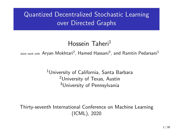
Quantized Decentralized Stochastic Learning over Directed Graphs Hossein Taheri 1 Joint work with Aryan Mokhtari 2 , Hamed Hassani 3 , and Ramtin Pedarsani 1 1 University of California, Santa Barbara 2 University of Texas, Austin 3 University of Pennsylvania Thirty-seventh International Conference on Machine Learning (ICML), 2020 1 / 30
Decentralized Optimization Decentralized Stochastic Learning involves multiple agents or nodes that collect data, and want to learn an ML model collaboratively. 2 / 30
Decentralized Optimization Decentralized Stochastic Learning involves multiple agents or nodes that collect data, and want to learn an ML model collaboratively. Applications including federated learning, multi-agent robotics systems, sensor networks, etc. 3 / 30
Decentralized Optimization Decentralized Stochastic Learning involves multiple agents or nodes that collect data, and want to learn an ML model collaboratively. Applications including federated learning, multi-agent robotics systems, sensor networks, etc. In many cases, communication links are asymmetric due to failures and bottlenecks and communication is done over a directed graph [Tsianos et al. 2012, Nedic et al. 2014, Assran et al. 2020]. 4 / 30
This Talk Link failure: Nodes communicate over a directed graph High communication cost: Nodes communicate compressed information Q ( x ) Compression operator Q : R d → R d 5 / 30
Introduction: Push-sum Algorithm Decentralized optimization over directed graphs with exact communication: = � n x i ( t + 1) j =1 w ij x j ( t ) − α ( t ) ∇ f i ( z i ( t )) = � n y i ( t + 1) j =1 w ij y j ( t ) z i ( t + 1) = x i ( t + 1) / y i ( t + 1) 6 / 30
Introduction: Push-sum Algorithm Decentralized optimization over directed graphs with exact communication: = � n x i ( t + 1) j =1 w ij x j ( t ) − α ( t ) ∇ f i ( z i ( t )) = � n y i ( t + 1) j =1 w ij y j ( t ) z i ( t + 1) = x i ( t + 1) / y i ( t + 1) [Nedic et al. 2014] prove that for convex, Lipschitz objectives √ √ z i ( T )) − f ⋆ � = O (1 / and α ( t ) = O (1 / T ) ⇒ � f ( � T ) , � T z i ( T ) = 1 � t =1 z i ( t ) T 7 / 30
Introduction: Push-sum Algorithm Decentralized optimization over directed graphs with exact communication: = � n x i ( t + 1) j =1 w ij x j ( t ) − α ( t ) ∇ f i ( z i ( t )) = � n y i ( t + 1) j =1 w ij y j ( t ) z i ( t + 1) = x i ( t + 1) / y i ( t + 1) [Nedic et al. 2014] prove that for convex, Lipschitz objectives √ √ z i ( T )) − f ⋆ � = O (1 / and α ( t ) = O (1 / T ) ⇒ � f ( � T ) , � T z i ( T ) = 1 � t =1 z i ( t ) T How can we incorporate quantized message exchanging for this setting? 8 / 30
Proposed Algorithm: Quantized Push-sum We propose the quantized Push-sum algorithm for stochastic optimization q i ( t ) = Q ( x i ( t ) − � x i ( t )) for all nodes k ∈ N out and j ∈ N in do i i send q i ( t ) and y i ( t ) to k and receive q j ( t ) and y j ( t ) from j . � x j ( t + 1) = � x j ( t ) + q j ( t ) end for x i ( t + 1) + � v i ( t + 1) = x i ( t ) − � w ij � x j ( t + 1) j ∈N in y i ( t + 1) = � i w ij y j ( t ) j ∈N in i z i ( t + 1) = v i ( t + 1) / y i ( t + 1) x i ( t + 1) = v i ( t + 1) − α ( t + 1) ∇ F i ( z i ( t + 1)) 9 / 30
Proposed Algorithm: Quantized Push-sum We propose the quantized Push-sum algorithm for stochastic optimization q i ( t ) = Q ( x i ( t ) − � x i ( t )) for all nodes k ∈ N out and j ∈ N in do i i send q i ( t ) and y i ( t ) to k and receive q j ( t ) and y j ( t ) from j . � x j ( t + 1) = � x j ( t ) + q j ( t ) end for x i ( t + 1) + � v i ( t + 1) = x i ( t ) − � w ij � x j ( t + 1) j ∈N in y i ( t + 1) = � i w ij y j ( t ) j ∈N in i z i ( t + 1) = v i ( t + 1) / y i ( t + 1) x i ( t + 1) = v i ( t + 1) − α ( t + 1) ∇ F i ( z i ( t + 1)) � x j ( t ) is stored in all out-neighbors of node j 10 / 30
Proposed Algorithm: Quantized Push-sum We propose the quantized Push-sum algorithm for stochastic optimization q i ( t ) = Q ( x i ( t ) − � x i ( t )) for all nodes k ∈ N out and j ∈ N in do i i send q i ( t ) and y i ( t ) to k and receive q j ( t ) and y j ( t ) from j . � x j ( t + 1) = � x j ( t ) + q j ( t ) end for x i ( t + 1) + � v i ( t + 1) = x i ( t ) − � w ij � x j ( t + 1) j ∈N in y i ( t + 1) = � i w ij y j ( t ) j ∈N in i z i ( t + 1) = v i ( t + 1) / y i ( t + 1) x i ( t + 1) = v i ( t + 1) − α ( t + 1) ∇ F i ( z i ( t + 1)) � x j ( t ) is stored in all out-neighbors of node j � x j ( t ) → x j ( t ) therefore q j ( t ) → 0 (Similar to [Koloskova et al. 2018] ) 11 / 30
Assumptions Assumptions on graph and connectivity 12 / 30
Assumptions Assumptions on graph and connectivity Strongly connected graph and W ij ≥ 0, W ii > 0 , ∀ i , j ∈ [ n ] 13 / 30
Assumptions Assumptions on graph and connectivity Strongly connected graph and W ij ≥ 0, W ii > 0 , ∀ i , j ∈ [ n ] Note that this results in � W t − φ 1 ′ � ≤ C λ t , ∀ t ≥ 1 where φ ∈ R n , 0 < λ < 1 14 / 30
Assumptions Assumptions on graph and connectivity Strongly connected graph and W ij ≥ 0, W ii > 0 , ∀ i , j ∈ [ n ] Note that this results in � W t − φ 1 ′ � ≤ C λ t , ∀ t ≥ 1 where φ ∈ R n , 0 < λ < 1 Assumptions on local objectives Lipschitz Local Gradients, � � � � � � � � � , ∀ x , y ∈ R d � ∇ f i ( y ) − ∇ f i ( x ) � ≤ L � y − x 15 / 30
Assumptions Assumptions on graph and connectivity Strongly connected graph and W ij ≥ 0, W ii > 0 , ∀ i , j ∈ [ n ] Note that this results in � W t − φ 1 ′ � ≤ C λ t , ∀ t ≥ 1 where φ ∈ R n , 0 < λ < 1 Assumptions on local objectives Lipschitz Local Gradients, � � � � � � � � � , ∀ x , y ∈ R d � ∇ f i ( y ) − ∇ f i ( x ) � ≤ L � y − x Bounded Stochastic Gradients, � � 2 � � ≤ D 2 , ∀ x ∈ R d � ∇ F i ( x , ζ i ) E ζ i ∼D i � 16 / 30
Assumptions Assumptions on graph and connectivity Strongly connected graph and W ij ≥ 0, W ii > 0 , ∀ i , j ∈ [ n ] Note that this results in � W t − φ 1 ′ � ≤ C λ t , ∀ t ≥ 1 where φ ∈ R n , 0 < λ < 1 Assumptions on local objectives Lipschitz Local Gradients, � � � � � � � � � , ∀ x , y ∈ R d � ∇ f i ( y ) − ∇ f i ( x ) � ≤ L � y − x Bounded Stochastic Gradients, � � 2 � � ≤ D 2 , ∀ x ∈ R d � ∇ F i ( x , ζ i ) E ζ i ∼D i � Bounded Variance, � � 2 � � ≤ σ 2 , ∀ x ∈ R d � ∇ F i ( x , ζ i ) − ∇ f i ( x ) E ζ i ∼D i � 17 / 30
Assumptions Assumption on quantization function The quantization function Q : R d → R d satisfies for all x ∈ R d , �� 2 � � � � ≤ ω 2 � x � 2 , � Q ( x ) − x (1) E Q � where 0 ≤ ω < 1. 18 / 30
Convergence Results (Convex objectives) 1 Define γ := � W − I � 2 and C ( λ, γ ) := � 6 C 2 (1 − λ )2 )(1+ γ 2 ) 6(1+ Theorem 1 Assume local objectives f i are convex for all i ∈ [ n ]. By choosing √ n ω ≤ C ( λ, γ ) and α = T , for all T ≥ 1, it holds that, √ 8 L � � � � T � 1 1 − f ⋆ = O z i ( t + 1) √ E f T nT t =1 19 / 30
Convergence Results (Convex objectives) 1 Define γ := � W − I � 2 and C ( λ, γ ) := � 6 C 2 (1 − λ )2 )(1+ γ 2 ) 6(1+ Theorem 1 Assume local objectives f i are convex for all i ∈ [ n ]. By choosing √ n ω ≤ C ( λ, γ ) and α = T , for all T ≥ 1, it holds that, √ 8 L � � � � T � 1 1 − f ⋆ = O z i ( t + 1) √ E f T nT t =1 Time average of local parameters z i converges to the exact solution! 20 / 30
Convergence Results (Convex objectives) 1 Define γ := � W − I � 2 and C ( λ, γ ) := � 6 C 2 (1 − λ )2 )(1+ γ 2 ) 6(1+ Theorem 1 Assume local objectives f i are convex for all i ∈ [ n ]. By choosing √ n ω ≤ C ( λ, γ ) and α = T , for all T ≥ 1, it holds that, √ 8 L � � � � T � 1 1 − f ⋆ = O z i ( t + 1) √ E f T nT t =1 Time average of local parameters z i converges to the exact solution! The convergence rate is the same as the case of undirected graphs with exact communication (e.g. [Yuan et al. 2016]) 21 / 30
Convergence Results (Convex objectives) 1 Define γ := � W − I � 2 and C ( λ, γ ) := � 6 C 2 (1 − λ )2 )(1+ γ 2 ) 6(1+ Theorem 1 Assume local objectives f i are convex for all i ∈ [ n ]. By choosing √ n ω ≤ C ( λ, γ ) and α = T , for all T ≥ 1, it holds that, √ 8 L � � � � T � 1 1 − f ⋆ = O z i ( t + 1) √ E f T nT t =1 Time average of local parameters z i converges to the exact solution! The convergence rate is the same as the case of undirected graphs with exact communication (e.g. [Yuan et al. 2016]) Error is proportional to 1 / √ n 22 / 30
Convergence Results (Non-Convex objectives) Theorem 2 √ n Let ω ≤ C ( λ, γ ) and α = T . Then after sufficiently large √ L number of iterations, ( T ≥ 4 n ), it holds that � � �� � � 2 � � T n � � 1 1 1 � � � ∇ f x i ( t ) = O √ E � � � T n nT t =1 i =1 23 / 30
Recommend
More recommend
Explore More Topics
Stay informed with curated content and fresh updates.
