Quantitative Justification for Third Natural . . . the Gravity - PowerPoint PPT Presentation
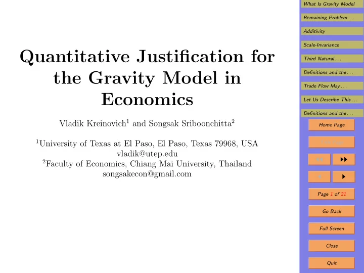
What Is Gravity Model Remaining Problem . . . Additivity Scale-Invariance Quantitative Justification for Third Natural . . . the Gravity Model in Definitions and the . . . Trade Flow May . . . Economics Let Us Describe This . . .
What Is Gravity Model Remaining Problem . . . Additivity Scale-Invariance Quantitative Justification for Third Natural . . . the Gravity Model in Definitions and the . . . Trade Flow May . . . Economics Let Us Describe This . . . Definitions and the . . . Vladik Kreinovich 1 and Songsak Sriboonchitta 2 Home Page 1 University of Texas at El Paso, El Paso, Texas 79968, USA Title Page vladik@utep.edu ◭◭ ◮◮ 2 Faculty of Economics, Chiang Mai University, Thailand songsakecon@gmail.com ◭ ◮ Page 1 of 21 Go Back Full Screen Close Quit
What Is Gravity Model Remaining Problem . . . 1. What Is Gravity Model Additivity • It is known that, in general: Scale-Invariance Third Natural . . . – neighboring countries trade more than distant ones, Definitions and the . . . and Trade Flow May . . . – countries with larger Gross Domestic Product Let Us Describe This . . . (GDP) g have a higher volume of trade. Definitions and the . . . • Thus, in general, the trade flow t ij between the two Home Page countries i and j : Title Page – increases when the GDPs g i and g j increase and ◭◭ ◮◮ – decreases with the distance r ij increases. ◭ ◮ • A qualitatively similar phenomenon occurs in physics: Page 2 of 21 the gravity force f ij between the two bodies: Go Back – increases when their masses m i and m j increase and Full Screen – decreases with the distance between then increases. Close Quit
What Is Gravity Model Remaining Problem . . . 2. What Is Gravity Model (cont-d) Additivity • Similarly, the potential energy e ij of the two bodies at Scale-Invariance distance r ij : Third Natural . . . Definitions and the . . . – increases when the masses increase and Trade Flow May . . . – decreases when the distance r ij increases. Let Us Describe This . . . • For the gravity force and for the potential energy, there Definitions and the . . . are simple formulas: Home Page f ij = G · m i · m j e ij = G · m i · m j ; . Title Page r 2 r ij ij ◭◭ ◮◮ • Both these formulas are a particular case of a general formula G · m i · m j ◭ ◮ . r α ij Page 3 of 21 • So, researchers use a similar formula to describe the Go Back dependence of the trade flow t ij on g i and r ij : t ij = G · g i · g j Full Screen . r α ij Close Quit
What Is Gravity Model Remaining Problem . . . 3. Remaining Problem and What We Do in This Additivity Talk Scale-Invariance • The formula t ij = G · g i · g j is known as the gravity Third Natural . . . r α ij Definitions and the . . . model in economics. Trade Flow May . . . • It has indeed been successfully used to describe the Let Us Describe This . . . trade flows between different countries. Definitions and the . . . Home Page • An analogy with gravity provides a qualitative expla- nation for the gravity model. Title Page • It is desirable to have a quantitative explanation as ◭◭ ◮◮ well. ◭ ◮ • Such an explanation is provided in this paper. Page 4 of 21 Go Back Full Screen Close Quit
What Is Gravity Model Remaining Problem . . . 4. Additivity Additivity • We would like to come up with a function F ( a, b, c ) for Scale-Invariance which t ij = F ( g i , g j , r ij ) . Third Natural . . . Definitions and the . . . • At first glance, the notion of a country seems to be Trade Flow May . . . very clear and well defined. Let Us Describe This . . . • However, there are many examples where this notion Definitions and the . . . is not that clear. Home Page • Sometimes, a country becomes a loose confederation of Title Page practically independent states. ◭◭ ◮◮ • In other cases, several countries form such a close trade ◭ ◮ union – from Benelux to European Union – that: Page 5 of 21 – most trade is regulated by the super-national or- Go Back gans Full Screen – and not by individual countries. Close Quit
What Is Gravity Model Remaining Problem . . . 5. Additivity (cont-d) Additivity • So, we have several different entities i 1 , . . . , i k , . . . , i ℓ Scale-Invariance located nearby forming a single super-entity. Third Natural . . . Definitions and the . . . • If we apply our formula to each individual entity i k , we Trade Flow May . . . get the expression t i k j = F ( g i k , g j , r i k j ) . Let Us Describe This . . . • Since all the entities i k are located close to each other, Definitions and the . . . we can assume that the distances r i k j are all the same: Home Page r i k j = r ij hence t i k j = F ( g i k , g j , r ij ) . Title Page • By adding these expressions, we get the trade flow be- ◭◭ ◮◮ tween the super-entity i and the country j : ◭ ◮ ℓ ℓ � � Page 6 of 21 t ij = t i k j = F ( g i k , g j , r ij ) . k =1 k =1 Go Back • Alternatively, we can treat the super-entity as a single Full Screen ℓ country with the overall GDP g i = � g i k . Close k =1 Quit
What Is Gravity Model Remaining Problem . . . 6. Additivity (cont-d) Additivity • In this case, by applying our formula, we get Scale-Invariance Third Natural . . . � ℓ � � Definitions and the . . . t ij = F ( g i , g j , r ij ) = F g i k , g j , r ij . Trade Flow May . . . k =1 Let Us Describe This . . . • Our estimate should not depend on whether we treat Definitions and the . . . this loose confederation a single country: Home Page F ( g i 1 , g j , r ij )+ . . . + F ( g i ℓ , g j , r ij ) = F ( g i 1 + . . . + g i ℓ , g j , r ij ) . Title Page ◭◭ ◮◮ • So, the function F ( a, b, c ) must be additive in a : ◭ ◮ F ( a, b, c ) + . . . + F ( a ′ , b, c ) = F ( a + . . . + a ′ , b, c ) . Page 7 of 21 • A similar argument can be make if we consider the case Go Back when j is a loose confederation of states, then: Full Screen F ( a, b, c ) + . . . + F ( a, b ′ , c ) = F ( a, b + . . . + b ′ , c ) . Close Quit
What Is Gravity Model Remaining Problem . . . 7. Scale-Invariance Additivity • The numerical value of the distance depends on what Scale-Invariance unit we use for measuring distance. Third Natural . . . Definitions and the . . . • For example, the distance in miles in different from the Trade Flow May . . . same distance in kilometers. Let Us Describe This . . . • If we replace the original unit with a λ times smaller Definitions and the . . . one, all numerical values multiply by λ : Home Page r ′ ij = λ · r ij . Title Page ◭◭ ◮◮ • It is reasonable to require that the estimates for the trade flow should not depend on what unit we use. ◭ ◮ Page 8 of 21 • Of course, we cannot simply require that F ( g i , g j , r ij ) = F ( g i , g j , λ · r ij ). Go Back • This would mean that the trade flow does not depend Full Screen on the distance at all. Close Quit
What Is Gravity Model Remaining Problem . . . 8. Scale-Invariance (cont-d) Additivity • This is OK, since: Scale-Invariance Third Natural . . . – the numerical value of the trade flow also depends Definitions and the . . . on what units we use: Trade Flow May . . . – we get different numbers if we use US dollars or Let Us Describe This . . . Thai Bahts. Definitions and the . . . • It is therefore reasonable to require that: Home Page – when we change the unit for measuring r ij , Title Page – then after an appropriate change t ij → t ′ ij = µ · t ij ◭◭ ◮◮ we get the same formula. ◭ ◮ • In other words, we require that for every λ > 0, there Page 9 of 21 exists a µ > 0 for which F ( g i , g j , λ · r ij ) = µ · F ( g i , g j , r ij ) . Go Back Full Screen • In other words, we require that Close F ( a, b, λ · c ) = µ · F ( a, b, c ) . Quit
What Is Gravity Model Remaining Problem . . . 9. Third Natural Property: Monotonicity Additivity • The final natural property is that: Scale-Invariance Third Natural . . . – as the distance increases, Definitions and the . . . – the trade flow should decrease. Trade Flow May . . . • In other words, the function F ( a, b, c ) should be a de- Let Us Describe This . . . creasing function of c . Definitions and the . . . Home Page • Now, we are ready to formulate our main result. Title Page ◭◭ ◮◮ ◭ ◮ Page 10 of 21 Go Back Full Screen Close Quit
What Is Gravity Model Remaining Problem . . . 10. Definitions and the Main Result Additivity • Definition 1. Scale-Invariance Third Natural . . . – A non-negative function F ( a, b, c ) is called additive Definitions and the . . . if the following two equalities hold: Trade Flow May . . . F ( a, b, c ) + . . . + F ( a ′ , b, c ) = F ( a + . . . + a ′ , b, c ); Let Us Describe This . . . F ( a, b, c ) + . . . + F ( a, b ′ , c ) = F ( a, b + . . . + b ′ , c ) . Definitions and the . . . Home Page – A function F ( a, b, c ) is called scale-invariant if for every λ , there exists a µ for which, for all a , b , c : Title Page F ( a, b, λ · c ) = µ · F ( a, b, c ) . ◭◭ ◮◮ – A function F ( a, b, c ) is called a trade function if it ◭ ◮ is additive, scale-invariant, and increasing in c . Page 11 of 21 • Proposition 1. Every trade function has the form Go Back F ( a, b, c ) = G · a · b for some constants G and α . Full Screen c α • Thus, we have indeed justified the gravity model. Close Quit
Recommend
More recommend
Explore More Topics
Stay informed with curated content and fresh updates.

