Quantifying Elephant Social Structure: Using a Bilinear Mixed - PowerPoint PPT Presentation

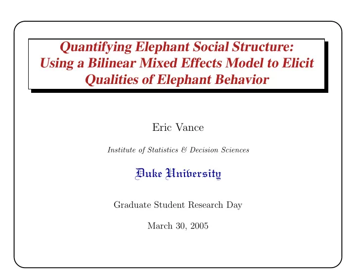
Quantifying Elephant Social Structure: Using a Bilinear Mixed Effects Model to Elicit Qualities of Elephant Behavior Eric Vance Institute of Statistics & Decision Sciences Duke University Graduate Student Research Day March 30, 2005

Elephant Social Structure • Only females form families. Males just run around looking to mate. • Oldest female is the leader since she is the largest and wisest. • Elephants within a family tend to be related.

Scientific Questions • Why do elephants stay in large groups even when food is scarce? • What role does genetics play in elephant social structure? • How does one quantify social structure in order to assess whether or not groups are larger in the Wet Season vs. the Dry Season?

Data Collection • Biologists in Kenya ride into the National Park looking for herds of elephants. • When a herd is spotted, they write down the names of the elephants present. • The biologists either stay to observe the family or move on to the next herd.

The Model • Data is binomial - y ij ∼ Bin( n ij , p ij ) - y ij is the number of times elephants i and j observed together. - n ij is the number of times either i or j observed. • Use a Generalized Linear Model = ⇒ Logistic regression - E ( y ij | θ ij ) = g ( θ ij ). - g is the inverse logit link function. - The probability of elephants i and j being together is: exp θ ij p ij = 1+exp θ ij . • θ ij is the linear predictor.

Linear Predictor θ ij How often are elephants together? • Intrinsic sociability a i . - Sociable elephants will be observed together with other elephants (in groups) more often than unsociable elephants. • Common intercept β 0 . • Genetic relatedness β g g ij . - DNA samples lead to a measure g ij of how closely elephant i and j are related. • Normal error γ ij (unexplained error or white noise). • Pairwise effect z ′ i z j between elephants i and j . θ ij = ( 1 2 β 0 + a i ) + ( 1 2 β 0 + a j ) + β g g ij + γ ij + z ′ i z j

Pairwise Effect z ′ i z j is the inner product of the positions of elephants i and j in “Social Space”. • For visual interpretability I choose the dimension of social space k = 2. Elephants i and j have positions z i and z j in 2D social space. z i ∼ N ( 0 , σ 2 z I) Zi z j ∼ N ( 0 , σ 2 z I) Zj • If z ′ i z j = 0 then elephants i and j interact as often as their sociabilities a i , a j and their genetics g ij would predict. • If z ′ i z j > 0 then i and j like each other and are observed together more often than the model would otherwise predict. • If z ′ i z j < 0 then i and j dislike each other.

Elephant Family Results

Posterior Intercepts β 0 Dry Genetics 1.2 Dry Season Wet Genetics Wet Season 1.0 0.8 0.6 0.4 0.2 0.0 −1 0 1 2 3 θ ij = ( 1 2 β 0 + a i ) + ( 1 2 β 0 + a j ) + β g g ij + γ ij + z ′ i z j

Posterior Sociabilities ¯ a 0.6 0.6 Dry Dry Genetics 0.4 0.4 AmbAud Amy Alt 0.2 0.2 Amb Aga Ang Aud Ang Alt Aga 0.0 0.0 Amy AmeAnh AmeAnh −0.2 −0.2 Ali Ast Ali −0.4 −0.4 Ast −0.6 −0.6 2 4 6 8 10 2 4 6 8 10 0.6 0.6 Wet Wet Genetics Aud 0.4 0.4 Ang AmyAng Aud 0.2 0.2 Alt Anh 0.0 0.0 AmeAnh Amb Ali Ast Ame Ali Amy Aga Alt −0.2 −0.2 Ast Aga Amb −0.4 −0.4 −0.6 −0.6 2 4 6 8 10 2 4 6 8 10 θ ij = ( 1 2 β 0 + a i ) + ( 1 2 β 0 + a j ) + β g g ij + γ ij + z ′ i z j

Posteriors for Genetic Coefficients β g 0.8 Dry Season Wet Season 0.6 0.4 0.2 0.0 0 1 2 3 4 5 6 θ ij = ( 1 2 β 0 + a i ) + ( 1 2 β 0 + a j ) + β g g ij + γ ij + z ′ i z j

Dry Season Social Space ¯ z i Posteriors Amy Dry Amb Ang Aud 0.5 0.0 Alt Anh Aga Ame Ali −0.5 Ast −0.5 0.0 0.5 θ ij = ( 1 2 β 0 + a i ) + ( 1 2 β 0 + a j ) + β g g ij + γ ij + z ′ i z j

Social Space Posterior Means ¯ z i 1.5 1.5 Dry Dry Genetics 1.0 1.0 Amy Amb Ang Amy Aud Aud 0.5 0.5 Ang Amb Aga Alt 0.0 Alt 0.0 Aga Anh Ame Ame Ali Ast Anh Ali −0.5 −0.5 Ast −1.0 −1.0 −1.5 −1.5 −1.5 −1.0 −0.5 0.0 0.5 1.0 1.5 −1.5 −1.0 −0.5 0.0 0.5 1.0 1.5 Aud 1.5 1.5 Ang Amy Amy Ang Aud 1.0 1.0 Aga Aga Alt Alt 0.5 Amb 0.5 Amb 0.0 0.0 Ame Anh Ame −0.5 −0.5 Anh Ali Ast −1.0 −1.0 Ast Ali Wet Wet Genetics −1.5 −1.5 −1.5 −1.0 −0.5 0.0 0.5 1.0 1.5 −1.5 −1.0 −0.5 0.0 0.5 1.0 1.5 θ ij = ( 1 2 β 0 + a i ) + ( 1 2 β 0 + a j ) + β g g ij + γ ij + z ′ i z j

Conclusions • Some of the posterior sociabilities in Family AA change depending on the season. • Posterior intercepts β 0 for the Wet seasons are greater than in the Dry seasons, indicating that the elephants are more gregarious during the Wet season. • Genetic coefficients β g > 0 for both Wet and Dry seasons. • There are clusters of elephants in social space.

Amy, Matriarch of Family AA

Binomial Data Example The total number of times data were recorded: Dry Season: N Dry = 331 Wet Season: N Wet = 171 If Amy, Ang, and Ali are observed together, and the others are missing, then: y AmyAng = y AmyAli = y AngAli = 1 n AmyAng = n AmyAli = n AngAli = 1 While for one missing elephant: y AmyAme = 0 n AmyAme = 1 Whereas for two missing elephants: y AstAme = 0 n AstAme = 0

Binomial Data, Cont. In this example of five elephants Amy, Angelina, Alison, Astrid, and Amelia at time = t , the y matrix of successful observations would be: Amy Ang Ali Ast Ame ... Amy 1 1 0 0 ... Ang 1 1 0 0 y t = ... Ali 1 1 0 0 ... Ast 0 0 0 0 ... Ame 0 0 0 0 Amy Ang Ali Ast Ame ... Amy 1 1 1 1 ... Ang 1 1 1 1 The n t matrix of potential observations = ... Ali 1 1 1 1 ... Ast 1 1 1 0 ... Ame 1 1 1 0

Pairwise Effect, Cont. • Only the inner products of the vectors z ′ i z j , z ′ i z k , z ′ j z k matter. Reflections or rotations of Social Space do not change inner products. Zk Zi Zi Zj Zj Zj Zk Zi Zk Social Space Reflection Rotation • All 3 social spaces are equivalent.

Procrustean Transformation • The posterior draws of the social space vectors must be reflected or rotated to give a coherent picture of the posterior distribution. 3 3 Dry Dry Wet Wet 2 2 Amy 1 1 Amy Amy Amy 0 0 −1 −1 −2 −2 −3 −3 Z ∗ transformed social space −3 −2 −1 0 1 2 3 −3 −2 −1 0 1 2 3 Z social space • Fix an arbitrary matrix Z 0 of positions in social space, then apply the Procrustean transformation: Z ∗ = Z 0 Z ′ ( ZZ ′ 0 Z 0 Z ′ ) − 1 2 Z

Vague Priors θ ij = ( 1 2 β 0 + a i ) + ( 1 2 β 0 + a j ) + β g g ij + γ ij + z ′ i z j Intercept: β 0 ∼ N (0 , 100) a i , a j ∼ N (0 , σ 2 σ 2 Sociabilities: soc ) , soc ∼ IG ( 1 2 , 1 2 ) Genetic Coefficient: β g ∼ N (0 , 100) γ ij ∼ N (0 , σ 2 σ 2 Pairwise error: γ ) , γ ∼ IG ( 1 2 , 1 2 ) � � σ 2 0 z σ 2 Social space: z i , z j ∼ N ( 0 , ) , z ∼ IG ( 1 2 ) 2 , 1 σ 2 0 z

Parameter Estimation Proceed using Gibbs sampling. For details see Peter Hoff’s article “Bilinear Mixed-Effects Models for Dyadic Data” in the current March 2005 issue of JASA .

Amy Sociability MCMC Dry Season Dry Season with Genetics 1.5 1.5 1.0 1.0 0.5 0.5 0.0 0.0 −0.5 −0.5 −1.0 −1.0 −1.5 −1.5 0 500 1000 1500 0 500 1000 1500 Wet Season Wet Season with Genetics 1.5 1.5 1.0 1.0 0.5 0.5 0.0 0.0 −0.5 −0.5 −1.0 −1.0 −1.5 −1.5 0 500 1000 1500 0 500 1000 1500

Amy Sociability Posterior Density Wet Genetics Dry Genetics 1.5 Wet Season Dry Season 1.0 0.5 0.0 −1.0 −0.5 0.0 0.5 1.0

Posterior Sociabilities a i Amy Amber 1.5 1.5 1.0 1.0 0.5 0.5 0.0 0.0 −1.5 −1.0 −0.5 0.0 0.5 1.0 1.5 −1.5 −1.0 −0.5 0.0 0.5 1.0 1.5 Astrid Amelia 1.5 1.5 1.0 1.0 0.5 0.5 0.0 0.0 −1.5 −1.0 −0.5 0.0 0.5 1.0 1.5 −1.5 −1.0 −0.5 0.0 0.5 1.0 1.5

Three Elephants’ Social Space Posterior Draws 3 Wet Wet Genetics 2 Amy Amy 1 Y coordinate 0 Ame Ame Ali −1 Ali −2 −3 −3 −2 −1 0 1 2 3 X coordinate

Posterior Innerproducts z ′ i z j 2 2 1 1 Amy Amy Ang Ame 0 0 −1 −1 −2 −2 −2 −1 0 1 2 −2 −1 0 1 2 2 2 1 1 Amy 0 0 Ali Ali Ast −1 −1 −2 −2 −2 −1 0 1 2 −2 −1 0 1 2

Posterior Normal Error σ 2 γ Wet Genetics Wet Season 10 Dry Genetics Dry Season 8 6 4 2 0 0.0 0.2 0.4 0.6 0.8 1.0 θ ij = ( 1 2 β 0 + a i ) + ( 1 2 β 0 + a j ) + β g g ij + γ ij + z ′ i z j

Pickiness in Social Space • When an elephant is farther from the origin in social space, the inner product term increases and has a larger influence in the model. • An elephant close to the origin will have a small pairwise effect in the model. • Pickiness is defined as the length of the vector in social space | z i | . Zi Zj • Elephant i is “pickier” than elephant j .

Amy’s Posterior Pickiness 1.0 1.0 Dry Season Wet Season 0.8 0.8 0.6 0.6 0.4 0.4 0.2 0.2 0.0 0.0 0 1 2 3 4 5 6 0 1 2 3 4 5 6 1.0 1.0 Dry Genetics Wet Genetics 0.8 0.8 0.6 0.6 0.4 0.4 0.2 0.2 0.0 0.0 0 1 2 3 4 5 6 0 1 2 3 4 5 6