Quadratic Video Interpolatoin Project page: - PowerPoint PPT Presentation
Quadratic Video Interpolatoin Project page: https://sites.google.com/view/xiangyuxu/qvi_nips19 Xiangyu Xu 1* Siyao Li 2* Wenxiu Sun 2 Qian Yin 3 Ming-Hsuan Yang 4 1 Carnegie Mellon University 2 SenseTime 3 Beijing Normal University 4 University of
Quadratic Video Interpolatoin Project page: https://sites.google.com/view/xiangyuxu/qvi_nips19 Xiangyu Xu 1* Siyao Li 2* Wenxiu Sun 2 Qian Yin 3 Ming-Hsuan Yang 4 1 Carnegie Mellon University 2 SenseTime 3 Beijing Normal University 4 University of California, Merced
Problem statement Temporal upsampling: how to interpolate between existing frames? ? … … … … 𝐽 𝑢 𝐽 0 𝐽 1 Time
Previous methods Flow-based Kernel-based Liu et al, Video frame synthesis using deep voxel flow, ICCV17 Niklaus et al, Video Frame Interpolation via Adaptive Convolution, CVPR17 Jiang et al, Super SloMo: High Quality Estimation of Multiple Niklaus et al, Video Frame Interpolation via Adaptive Separable Convolution, Intermediate Frames for Video Interpolation, CVPR18 ICCV17 Existing methods usually assume linear motion . However, the motion in real scenarios can be more complex and nonlinear ! Phase-based Meyer et al, Phase-Based Frame Interpolation for Video, CVPR15 Meyer et al, PhaseNet for Video Frame Interpolation, CVPR18
Motivation result of the state-of-the-art method Jiang et al, CVPR18 result of our quadratic model Applying higher-order model to exploit the acceleration information from more neighboring frames.
Algorithm: overview f →− Quadratic 0 1 Flow flow reversal f prediction → 0 1 f f → t → Flow 0 t 0 Synthesis estimation f Quadratic → 1 0 Flow flow , , , I I I I reversal − 1 0 1 2 prediction f → I 1 2 f f → t → t 1 1 t 1. Quadratic flow prediction 2. Flow reversal layer 3. Synthesis
Algorithm: 1. quadratic flow prediction t → = + Equation of motion ( ) , f v a d d 0 0 t 0 0 With 𝑏 𝜐 = 𝐷 , we have = + + − 2 ( ) / 2 ( ) / 2 f f f t f f t → → →− → →− 0 0 1 0 1 0 1 0 1 t
Algorithm: 2. flow reversal layer While we have 𝑔 0→𝑢 from the last step, we need 𝑔 t→0 for frame warping. 𝑔 𝑔 0→𝑢 t→0 + − − (|| ( ) || )( ( )) w x f x u f x → → + 0 2 0 t t = ( ) ( ) x f x N u → ( ) f u 0 t → + − 0 t (|| ( ) || ) w x f x u → + 0 2 t ( ) ( ) x f x N u → 0 t
Algorithm: 3. synthesis Adaptive flow filtering (learnable “median filter”) The proposed flow filtering method: = + + ( ) ( ( )) ( ), f u f u u r u → → 0 0 t t where 𝜀 denotes the learned offset, and 𝑠 is the learned residual map. moving direction 𝐽 0 𝑔 Refined 𝑔 Refined 𝑔 t→0 t→0 t→0 by convolution by our method
Algorithm: 3. synthesis Warping and fusing frames 𝑔′ t→0 𝑔′ t→1 መ 𝐽 𝑢 𝐽 0 𝐽 1 ˆ ( ) = + − t t (1 ) , I u mI m I 0 1 t where 𝑛 is the learned mask for fusing the warped frames.
Results
Results The proposed method ranks the 1st in the ICCV 2019 video interpolation challenge. Method PSNR SSIM Ours 25.47 0.7383 NoFlow 25.05 0.7231 Team Eraser 24.58 0.7052 DAIN 24.56 0.7062 Team Eraser 24.55 0.7045 BOE_IOT_AIBE_IMP 24.41 0.6998 KAIST-VICLAB 23.93 0.6869 ZSFI 21.83 0.6094 baseline (overlay) 20.39 0.6625
Results Video examples:
Quadratic model Project Linear model Poster: East Exhibition Hall B+C #97 Time: 5:00-7:00 PM , Dec 12
Recommend
More recommend
Explore More Topics
Stay informed with curated content and fresh updates.
