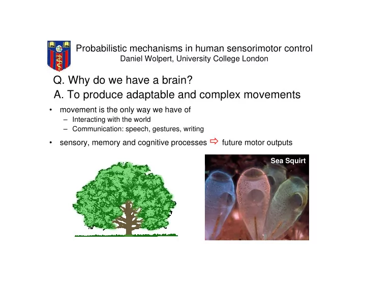
Q. Why do we have a brain? A. To produce adaptable and complex - PowerPoint PPT Presentation
Probabilistic mechanisms in human sensorimotor control Daniel Wolpert, University College London Q. Why do we have a brain? A. To produce adaptable and complex movements movement is the only way we have of Interacting with the world
Probed distributions and optimal means Distributions Possible Loss functions MODE ρ =0.2 Maximize Hits -2 -1 0 1 2 Error (cm) MEDIAN ρ =0.3 = Loss error MEAN ρ =0.5 = 2 Loss ( ) error ρ =0.8 Robust estimator -2 -1 0 1 2 Error (cm)
Shift of mean against asymmetry (n=8) Mean squared error with robustness to outliers
Personalised loss function = ∑ error α Loss i α= 0.1 1.0 1.3 1.5 1.7 1.9 2.1 2.3 2.5 2.7 2.9 3.1 3.3 3.5 3.7 3.9
Bayesian decision theory Increasing probability of avoiding keeper Increasing probability of being within the net
Imposed loss function (Trommershäuser et al 2003) +100 +100 -100 -500 0 +100
Optimal performance with complex regions
State estimation • State of the body/world – Set of time-varying parameters which together with • Dynamic equations of motion • Fixed parameters of the system (e.g. mass) – Allow prediction of the future behaviour • Tennis ball – Position – Velocity – Spin
State estimation NOISE Observer NOISE
Kalman filter • Minimum variance estimator – Estimate time-varying state – Can’t directly observe state but only measurement + = + + x x u w A B 1 t t t t + = + y x v C 1 t t t + = + + − ˆ ˆ ˆ x x u [ y x ] A B K C 1 t t t t t t
State estimation + = + + − ˆ ˆ ˆ x x u [ y x ] A B K C � � �� � 1 t t t t t t ForwardDynamicModel
Kalman Filter • Optimal state estimation is a mixture – Predictive estimation (FF) – Sensory feedback (FB)
Eye position Location of object based on retinal location and gaze direction Percept Actual Motor command Eye FM Position
Sensory likelihood ∝ P(state| sensory input) P(sensor yinput|s tate ) P(st ate ) (Wolpert & Kawato, Neural Networks 1998 Haruno, Wolpert, Kawato, Neural Computation 2001)
Sensory prediction Our sensors report • Afferent information: changes in outside world • Re-afferent information: changes we cause = + Internal External source source
Tickling Self-administered tactile stimuli rated as less ticklish than externally administered tactile stimuli. (Weiskrantz et al, 1971)
Does prediction underlie tactile cancellation in tickle? 3 2.5 Tickle rating rank P<0.001 2 Gain control or precise 1.5 spatio-temporal prediction? 1 0.5 0 Self-produced Robot-produced tactile stimuli tactile stimuli Condition
Spatio-temporal prediction 4 4 P<0.001 3.5 3.5 P<0.001 Tickle rating rank 3 P<0.001 3 Tickle rating rank P<0.001 2.5 2.5 2 2 1.5 1.5 1 1 0.5 0.5 0 0 Delay 0ms Delay Delay Delay Robot- 0 degrees 30 degrees 60 degrees 90 degrees External 100ms 200ms 300ms produced Condition tactile stimuli Condition (Blakemore, Frith & Wolpert. J. Cog. Neurosci. 1999)
The escalation of force
Tit-for-tat Force escalates under rules designed to achieve parity: Increase by ~40% per turn (Shergill, Bays, Frith & Wolpert, Science, 2003)
Perception of force 70% overestimate in force
Perception of force
Labeling of movements discrepancy sensory Large
Defective prediction in patients with schizophrenic Patients Controls • The CNS predicts sensory consequences • Sensory cancellation in Force production • Defects may be related to delusions of control
Motor Learning Required if: • organisms environment, body or task change • changes are unpredictable so cannot be pre-specified • want to master social convention skills e.g writing Trade off between: – innate behaviour (evolution) • hard wired • fast • resistant to change – learning (intra-life) • adaptable • slow • Maleable
Actual behaviour Motor Learning
Supervised learning is good for forward models Predicted outcome can be compared to actual outcome to generate an error
Weakly electric fish (Bell 2001) Produce electric pulses to • recognize objects in the dark or in murky habitats • for social communication. The fish electric organ is composed of electrocytes, • modified muscle cells producing action potentials • EOD = electric organ discharges • Amplitude of the signal is between 30 mV and 7V • Driven by a pacemaker in medulla, which triggers each discharge
Sensory filtering Skin receptors are derived from the lateral line system Removal of expected or predicted sensory input is one of the very general functions of sensory processing. Predictive/associative mechanisms for changing environments
Primary afferent terminate in cerebellar-like structures Primary afferents terminate on principal cells either directly or via interneurons
Block EOD discharge with curare Specific for Timing (120ms), Polarity, Amplitude & Spatial distribution
Proprioceptive Prediction Tail bend affects feedback Passive Bend phase locked to stimulus: Bend
Learning rule Changes in synaptic strength requires principal cell spike discharge Change depends on timing of EPSP to spike Anti-Hebbian learning T1 T2 T2-T1 • Forward Model can be learned through self-supervised learning • Anti-hebbian rule in Cerebellar like structure of he electric fish
Motor planning (what is the goal of motor control) • Tasks are usually specified at a symbolic level • Motor system works at a detailed level, specifying muscle activations • Gap between high and low-level specification • Any high level task can be achieved in infinitely many low-level ways Duration Hand Trajectory Joint Muscles
Motor evolution/learning results in stereotypy Stereotypy between repetitions and individuals Eye-saccades Arm- movements Time (ms) • 2/3 power law • Main sequence • Fitts’ law • Donder’s law • Listings Law
Models HOW models – Neurophysiological or black box models – Explain roles of brain areas/processing units in generating behavior WHY models – Why did the How system get to be the way it is? – Unifying principles of movement production • Evolutionary/Learning – Assume few neural constraints
The Assumption of Optimality Movements have evolved to maximize fitness – improve through evolution/learning – every possible movement which can achieve a task has a cost – we select movement with the lowest cost Overall cost = cost 1 + cost 2 + cost 3 ….
Optimality principles • Parsimonious performance criteria � Elaborate predictions • Requires – Admissible control laws – Musculoskeletal & world model – Scalar quantitative definition of task performance – usually time integral of f(state, action)
Open-loop • What is the cost – Occasionally task specifies cost • Jump as high as possible • Exert maximal force – Usually task does not specify the cost directly • Locomotion well modelled by energy minimization • Energy alone is not good for eyes or arms
What is the cost? Saccadic eye movements • little vision over 4 deg/sec • frequent 2-3 /sec • deprives us of vision for 90 minutes/day ⇒ Minimize time
Arm movements Movements are smooth – Minimum jerk (rate of change of acceleration) of the hand (Flash & Hogan 1985) ∫ ��� T = + 2 ��� 2 ( ) ( ) Cost x t y t dt 0 = + − τ − τ − τ 4 5 3 ( ) ( )(15 6 10 ) x t x x x 0 0 T = + − τ − τ − τ 4 5 3 ( ) ( )(15 6 10 ) y t y y y 0 0 T τ = / t T
Smoothness • Minimum Torque change (Uno et al, 1989) T ∫ � Elbow = τ + τ 2 2 � ( ) ( ) torque Cost t t dt s e 0 Shoulder torque
The ideal cost for goal-directed movement • Makes sense - some evolutionary/learning advantage • Simple for CNS to measure • Generalizes to different systems – e.g. eye, head, arm • Generalizes to different tasks – e.g. pointing, grasping, drawing → Reproduces & predicts behavior
Motor command noise Noise Motor Position System Error minimized by rapidity
Fundamental constraint=Signal-dependent noise • Signal-dependent noise: – Constant coefficient of variation – SD (motor command) ~ Mean (motor command) • Evidence from – Experiments: SD (Force) ~ Mean (Force) – Modelling • Spikes drawn from a renewal process • Recruitment properties of motor units (Jones, Hamilton & Wolpert , J. Neurophysiol., 2002)
Task optimization in the presence of SDN An average motor command ⇒ probability distribution (statistics) of movement. Controlling the statistics of action Controlling the statistics of action Given SDN, Task ≡ ≡ optimizing optimizing f(statistics f(statistics) ) Given SDN, Task
Finding optimal trajectories for linear systems Impulse response Signal-dependent noise p(t) System σ = 2 2 2 ( ) ( ) u t k u t time T M ∫ M = τ − τ τ = [ ( )] ( ) ( ) E x M u p M d A A 0 Constraints x(t) ∫ M ( ) = τ ( ) − τ τ = [ ( )] ( ) ( ) 0 n n E x M u p M d 0 time ∫ M ∫ M = τ − τ τ = τ − τ τ 2 [ ( )] [ ( ) ( )] [ ( )] ( ) Var x T Var u p T d Var u p T d Cost 0 0 ∫ M ∫ M = τ − τ τ = τ τ τ 2 2 2 2 ( ) ( ) ( ) ( ) k u p T d w u d 0 0 Linear constraints with quadratic cost: can use quadratic programming or isoperimetric optimization
Saccade predictions 3rd order linear system SDN Motor Jerk command
Prediction: very slow saccade 22 degree saccade in 270 ms (normally ~ 70 ms) 20 Degrees 0 0 100 200 Time (ms)
Head free saccade Τ 1=0.15 Τ 2=0.08 Free parameter, eye:head noise Τ 1=0.3 Τ 2=0.3 120 120 100 100 Gaze Gaze 80 80 Head Degrees Head Degrees 60 60 40 40 Eye 20 Eye 20 0 0 0 100 200 300 400 500 600 700 800 0 100 200 300 400 500 600 700 800 Time (ms) Time (ms) (Tomlinson & Bahra, 1986)
Coordination: Head and eye For a fixed duration (T), Var(A)=k A 2 Eye only Head only Eye & Head Var(A)= k (A/2) 2 + k (A/2) 2 Var(A)=k A 2 Var(A)=k A 2 = k A 2 /2
Movement extent vs. target eccentricity 120 } } 100 80 60 Head 40 20 Eye 0 0 100 200 300 400 500 600 700 800 Angular deviation at 100 90 80 Head 70 acquisition 60 50 40 30 Eye 20 10 0 0 20 40 60 80 100 120 140 Gaze amplitude Gaze amplitude
Arm movements Smoothness Non smooth movement ⇒ requires abrupt change in velocity ⇒ given low pass system ⇒ large motor command ⇒ increased noise Smoothness ⇒ accuracy Drawing ( ⅔ power law) f=path error Obstacle avoidance f= limit probability of collision Feedforward control •Ignores role of feedback •Generates desired movements •Cannot model trial-to-trial variability
Optimal feedback control (Todorov 2004) – Optimize performance over all possible feedback control laws – Treats feedback law as fully programmable • command=f(state) • Models based on reinforcement learning optimal cost-to-go functions • Requires a Bayesian state estimator
Minimal intervention principle • Do not correct deviations from average behaviour unless they affect task performance – Acting is expensive • energetically • noise – Leads to • uncontrolled manifold • synergies U n c o n t r o l l e d m a n i f o l d
Optimal control with SDN • Biologically plausible theoretical underpinning for both eye, head, arm movements • No need to construct highly derived signals to estimate the cost of the movement • Controlling statistics in the presence of noise
What is being adapted? • Possible to break down the control process: • Visuomotor rearrangements • Dynamic perturbations • [timing, coordination , sequencing] • Internal models captures the relationship between sensory and motor variables
Altering dynamics
Altering Kinematics
Representation of transformations Non-physical Physical Look-up Parameters Parameters Table θ =f(x ,ω ) θ =acos(x/L) x x x x θ ÷ 1 10 L L 3 35 θ . . . . asin θ θ High storage Low storage High flexibility Low flexibility Low Generalization High Generalization
Generalization paradigm • Baseline – Assess performance over domain of interest – (e.g. workspace) • Exposure – Perturbation: New task – Limitation: Limit the exposure to a subdomain • Test – Re-assess performance over entire domain of interest
Difficulty of learning (Cunningham 1989, JEPP-HPP) • Rotations of the visual field from 0—180 degrees Difficulty • increases from 0 to 90 • decreases from 120 to 180 • What is the natural parameterization
Viscous curl field (Shadmehr & Mussa-Ivaldi 1994, J. Neurosci.)
Representation from generalization: Dynamic 1. Test: Movements over entire workspace 2. Learning – Right-hand workspace – Viscous field 3. Test: Movements over left workspace Two possible interpretations Left hand workspace force = f(hand velocity) Before After with Cartesian field or torque=f(joint velocity) Joint-based learning of dynamics (Shadmehr & Mussa-Ivaldi 1994, J. Neurosci.)
Visuomotor coordinates Cartesian Spherical Polar Joint angles z (x,y,z) (α 1 ,α 2 ,α 3 ) z ( r, φ,θ) y θ r x α 3 φ α 1 α 2 y x
Representation- Visuomotor 1. Test: Pointing accuracy to a set of targets 2. Learning – visuomotor remapping – feedback only at one target 3. Test: Pointing accuracy to a set of targets Predictions of eye-centred spherical coordinates Predict ion of ey e- ce nt red sphe rical coordinat es y = 22.2/ 16.2 cm y = 36.2 cm y = 29.2/ 26.2 cm - 30 - 40 - 50 z = - 43.6 cm z = - 35.6 cm z = - 27.6 cm 40 30 (Vetter et al, J. Neurophys, 1999) 20 - 20 - 10 0 10 20 - 20 - 10 0 10 20 - 20 - 10 0 10 20 x (cm ) • Generalization paradigms can be used to assess – Extent of generalization – Coordinate system of transformations
Altering dynamics: Viscous curl field Before Early with force Late with force Removal of force
Recommend
More recommend
Explore More Topics
Stay informed with curated content and fresh updates.
