Q -Gorenstein deformation families of Fano varieties or The - - PowerPoint PPT Presentation

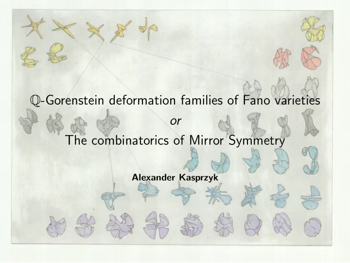
Q-Gorenstein deformation families of Fano varieties

• r

The combinatorics of Mirror Symmetry

Alexander Kasprzyk

Fano manifolds

Smooth varieties, called manifolds, come with a natural notion of curvature, and fall into one of three classes. Negative curvature Flat Positive curvature General type Calabi–Yau Fano There are finitely many Fano manifolds in each dimension.

Fano manifolds: Basic building blocks of geometry Fano manifolds are the building blocks from which other varieties are formed.

Both from the Minimal Model Program And in terms of explicit constructions

Fano art by Gemma Anderson

Fano manifolds: Classification

The classification of Fano manifolds is known up to dimension 3. Dimension 1:

P1 (i.e. the Reimann sphere)

Dimension 2 (del Pezzo, 1880s):

P2 P1 × P1 The blow-up of P2 in at most 8 points.

These are called del Pezzo surfaces. Dimension 3 (Mori–Mukai, 1980s):

105 cases

Very little is known in dimension ≥ 4.

Fano polytopes and toric geometry

Fix a lattice N ≅ Zn. A convex lattice polytope P ⊂ N ⊗Q = NQ is Fano if: dim(P) = n; 0 ∈ int(P); each v ∈ vert(P) is a primitive lattice point of N. Two Fano polytopes P and Q are considered to be isomorphic if there exists a change of basis of N sending P to Q. That is, P ≅ Q ⇐ ⇒ ϕ(P) = Q, for some ϕ ∈ GLn(Z) ≅ via ϕ ∶ e1 ↦ e1 e2 ↦ e1 − e2 We consider Fano polytopes only up to isomorphism.

Fano polytopes and toric geometry

To a Fano polytope P ⊂ NQ we associate the spanning fan. The spanning fan describes a toric Fano variety XP. ← → ← → XP = P2 The geometry of XP is encoded in the combinatorics of P. For example, the singularities of XP can be read off P.

Toric Fano manifolds: Classification

A Fano polytope P is smooth if: For each facet F of P, vert(F) are a Z-basis of N. n-dimensional toric Fano smooth Fano polytope P manifold X with dim(P) = n

toric geometry

←

• →

Dimension 2:

P2; P1 × P1; the blow-up of P2 in at most 3 points.

Toric Fano manifolds: Classification

Being toric is unusual: Dimension 2:

5 of the 10 del Pezzo surfaces are toric.

Dimension 3:

18 of the 105 Fano manifolds are toric.

But being toric is good: we can use the combinatorics of lattice polytopes to study them. For example, Øbro (2007) gave an efficient algorithm for classifying smooth Fano polytopes in any dimension. Dimension 1 2 3 4 5 6 7 8 Number 1 5 18 124 866 7 622 72 256 749 892 They grow slowly – approximately by a power of 10 per dimension.

Mirror Symmetry

n-dimensional Fano Laurent polynomial f manifold X in n variables

Mirror Symmetry

←

• →

f = x + y + z + 1 xyz deformation

• →
• →

Newt(f ) n-dimensional toric Fano polytope P Fano variety XP with dim(P) = n

toric geometry

←

• →

Example: P2

Illustrate this equivalence in the case of X = P2. We start with the Laurent polynomial f = x + y + 1 xy ∈ C[x±1,y±1] Associated with f is its period πf (t) = ( 1 2πi )

2

∫∣x∣=∣y∣=1 1 1 − tf dx x dy y , t ∈ C,∣t∣ ≪ ∞. The Taylor expansion of the period has coefficients given by the constant term of successive powers of f πf (t) = ∑

k≥0

coeff1(f k)tk = 1 + 6t3 + 90t6 + 34650t9 + 756756t12 + 17153136t15 + ... = ∑

k≥0

(3k)! (k!)3 t3k

Example: P2

πf (t) = 1 + 6t3 + 90t6 + 34650t9 + 756756t12 + 17153136t15 + ... The coefficients of πf agree with certain Gromov–Witten invariants of X. Roughly speaking, they count curves in X with given degree and a certain constraint on the C-structure. This is called the regularised quantum period ̂ GX.

f is mirror dual to X if πf = ̂ GX

The Newton polytope P ⊂ NQ of f gives a toric Fano variety XP Q-Gorenstein deformation equivalent to X. In this case we recover P2. f = x + y + 1 xy P = Newt(f ) = ⊂ NQ

Example: P2

The mirror f for X is typically not unique. One way of transforming f to a mirror-equivalent Laurent polynomial g is via a mutation. This is a change of variables ϕ ∶ (C×)n ⇢ (C×)n such that g = ϕ∗f is a Laurent polynomial with the same period: πf (t) = πg(t) In the case f = x + y + 1

xy we can apply the mutation

ϕ ∶ x ↦ x 1 + x

y

y ↦ y 1 + x

y

Then: g = ϕ∗f = ϕ∗ (x + y + 1 xy ) = x 1 + x

y

+ y 1 + x

y

+ (1 + x

y ) 2

xy

Example: P2

g = ϕ∗f = x 1 + x

y

+ y 1 + x

y

+ (1 + x

y ) 2

xy = y(y + x) y + x + y2 + 2xy + x2 xy3 = y + 1 xy + 2 y2 + x y3 ∈ C[x±1,y±1] One can compute the period of g: πg(t) = 1 + 6t3 + 90t6 + 34650t9 + 756756t12 + ⋯ = πf (t)

g is also a mirror for P2

Mutation of a Laurent polynomial

A mutation of f ∈ C[x±1] requires two pieces of data: a grading on monomials; a factor F ∈ C[x±1]. The grading is a map w ∶ xa ↦ w(a) from monomials to Z. The factor is a Laurent polynomial with w(F) = {0} such that fh = F −hrh, for all h < 0, where rh ∈ C[x±1]. Here fh = “the terms of f in graded piece h”, i.e. w(fh) = {h}. Then ϕ ∶ xa ↦ xaF w(a) is a mutation of f with g = ϕ∗f = ∑

h<0

rh + ∑

h≥0

fhF h

Example: P2 Mutation is a combinatorial operation on the Newton polytopes

At the level of Newton polytopes we have transformed the Fano polygon for P2 into the Fano polygon for P(1,1,4): Newt(x + y + 1

xy ) =

• →

= Newt(y + 1

xy + 2 y2 + x y3 )

Notice that P(1,1,4) is a singular toric Fano variety. It has two smooth cones, and one singular cone corresponding to a 1

4(1,1) singularity.

Mutation of P ⊂ NQ

A mutation of P ⊂ NQ requires two pieces of data: a grading on N; a factor of P. The grading is given by a primitive lattice vector w ∈ M = Hom(N,Z). The factor is a convex lattice polytope F ⊂ w⊥ ⊂ NQ such that {v ∈ vert(P) ∣ w(v) = h} ⊂ (−h)F + Rh ⊂ Ph, for all h < 0, where Rh ⊂ NQ is a convex lattice polytope. Here Ph = conv(v ∈ P ∩ N ∣ w(v) = h). The the mutation of P is Q = conv(⋃

h<0

Rh ∪ ⋃

h≥0

(Ph + hF))

Mutation of P ⊂ NQ

In the example of P2 we pick w = (−1,−1) ∈ M, F = conv{(0,0),(1,−1)} ⊂ w⊥ ⊂ NQ. Then mutation adds or subtracts dilates of F depending on height:

• 2
• 1

1 2

• →
• 2
• 1

1 2

Example: P2

Now consider the dual polytope to P ⊂ NQ: P∗ = {u ∈ MQ ∣ u(v) ≥ −1 for all v ∈ P} NQ MQ P2 ∶

dual

• →
• →

P(1,1,4) ∶

dual

• →

Mutation of P∗ ⊂ MQ

Mutation acts via a piecewise GLn(Z) map on M: u → u − w min{w(v) ∣ v ∈ vert(F)} NQ MQ P2 ∶

dual

• →

( 2

1 −1 0)

(1

1)

• →
• →

P(1,1,4) ∶

dual

• →

Mutation of P∗ ⊂ MQ

P∗ =

• →

= Q∗ Mutation has straightened out the bottom-left corner of Q∗. Since this is a piecewise GLn(Z) map on M, we have that: Vol(P∗) = Vol(Q∗), Ehr(P∗) = Ehr(Q∗) Equivalently: (−KXP)n = (−KXQ)n, Hilb(XP,−KXP) = Hilb(XQ,−KXQ)

Mutation of Markov triples

We can continue mutating P2, moving from Fano triangle to Fano triangle:

(1,1,1) (1,1,2) (1,2,5) (2,5,29) (5,29,433) (2,29,169) (1,5,13) (5,13,194) (1,13,34)

The vertices (a,b,c) correspond to the Fano triangles for P(a2,b2,c2). The vertices (a,b,c) correspond to solutions to the Markov equation: a2 + b2 + c2 = 3abc

Mutation of Markov triples

A solution (a,b,c) ∈ Z3

>0 of the Markov equation

a2 + b2 + c2 = 3abc is called a Markov triple. All Markov triples can be obtained from (1,1,1) via mutation: (a,b,c) → (3bc − a,b,c) Mutations of the Markov triples correspond to mutations of the Fano triangles arising from P2.

Quiver mutation

We can associate a quiver QP to a Fano polygon P ⊂ NQ. We have a vertex vi for each edge Ei of P. Let wi ∈ M be the primitive (inner) normal vector to Ei. Then the number of arrows between vertices vi and vj is given by wi ∧ wj = det(wi wj), where the sign determines the orientation. For P2 we get: P = w1 = (−1,−1) w2 = (−1,2) w3 = (2,−1) QP =

v

1

v

2

v

3

3 3 3

Quiver mutation

We can mutate QP about a vertex vi. For every path vj → vi → vk add in a new edge vj → vk; Reverse the direction of every arrow that starts or ends at vi; Cancel opposing edges. We recover the quiver for P(1,1,4): P2 ∶

• →

v

1

v

2

v

3

3 3 3

• →
• →

P(1,1,4) ∶

• →

v

1

v

2

v

3

3 3 6

Mirrors for P2

P2 = ∶

v

1

v

2

v

3

3 3 3

• →

v

1

v

2

v

3

3 3 6

∶ = P(1,1,4) Notice that the quiver for P(1,1,4) isn’t balanced. We re-balance by adding multiplicities for to vertices vi given by the edge lengths Ei of the Fano polygon. Q(1,1,1) ∶

v

1

v

2

v

3

3 3 3 (1) (1) (1)

• →

v

1

v

2

v

3

3 3 6 (2) (1) (1)

∶ Q(1,1,2) This re-balancing condition is the Markov equation.

Mirrors for P2

We obtain a tree of quiver mutations

(1,1,1) (1,1,2) (1,1,2) (1,1,2) (1,2,5) (1,2,5) (1,2,5) (1,2,5) (a,b,c) (a,b,c) (a,b,c) (a,b,c) (a,b,c) (a,b,c) (a,b,c) (a,b,c) (a,b,c) (a,b,c) (a,b,c) (a,b,c) (1,2,5) (1,2,5)

where the quiver Q(a,b,c) corresponding to P(a2,b2,c2) is balanced via assigning weights a,b,c to the vertices v1,v2,v3. Here (a,b,c) is a solution to the Markov equation a2 + b2 + c2 = 3abc. This corresponds to the space of mirrors for P2 via Mirror Symmetry.