Project discussion, 22 May: Mandatory but ungraded. Thanks for doing - PowerPoint PPT Presentation

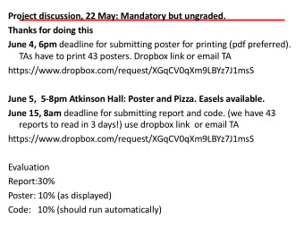
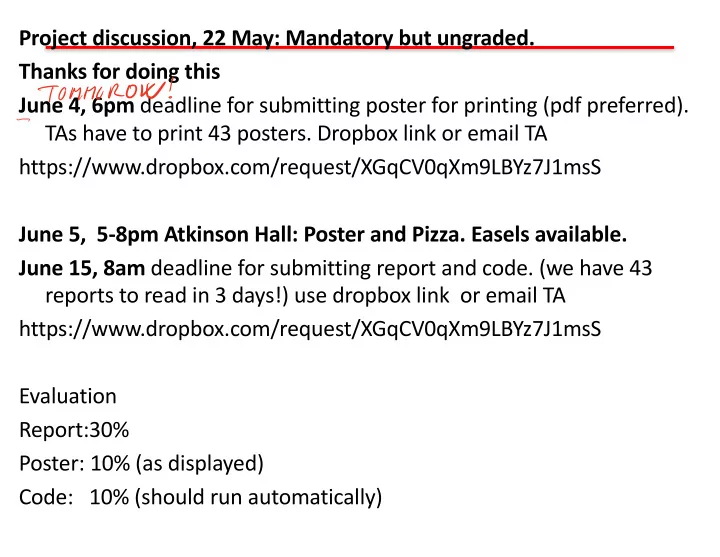
Project discussion, 22 May: Mandatory but ungraded. Thanks for doing this TOMMOROW June 4, 6pm deadline for submitting poster for printing (pdf preferred). TAs have to print 43 posters. Dropbox link or email TA https://www.dropbox.com/request/XGqCV0qXm9LBYz7J1msS June 5, 5-8pm Atkinson Hall: Poster and Pizza. Easels available. June 15, 8am deadline for submitting report and code. (we have 43 reports to read in 3 days!) use dropbox link or email TA https://www.dropbox.com/request/XGqCV0qXm9LBYz7J1msS Evaluation Report:30% Poster: 10% (as displayed) Code: 10% (should run automatically)

Beamforming / DOA estimation M I O O O N Mac to

o OO

We can’t model everything… so Reflection from complex geology Back scattering from fish school Detection of mines. Navy uses dolphins to assist in this. Dolphins = real ML! Predict acoustic field in turbulence Weather prediction

Machine Learning for physical Applications noiselab.ucsd.edu Murphy: “… the best way to make machines that can learn from data is to use the tools of probability theory , which has been the mainstay of statistics and engineering for centuries.“ 8

DOA estimation with sensor arrays x n e j 2 π X λ r m sin θ n y m = 1 2 M n -90 o N 90 o 1 k 2 N-1 � 1 � 2 2 � k 1 m ∈ [1 , · · · , M ]: sensor N-2 3 � n ∈ [1 , · · · , N ]: look direction 45 o -45 o y = Ax 0 o x 1 x 2 y = [ y 1 , · · · , y M ] T , x = [ x 1 , · · · , x N ] T p 1 ( r ,t) = x 1 ej( � t- k 1 r ) p 2 ( r ,t) = x 2 ej( � t- k 2 r ) A = [ a 1 , · · · , a N ] x ∈ C , θ ∈ [ − 90 � , 90 � ] 1 [ e j 2 π λ r 1 sin θ n , · · · , e j 2 π λ r M sin θ n ] T a n = √ k = − 2 π M λ sin θ , λ :wavelength The DOA estimation is formulated as a linear problem

Compressive beamforming O .: measurement vector ;: Transform matrix x : desired sparse vector 3: selection matrix A : measurement matrix Sparse: N> A Often N>>M In compressive beamforming 3 is given by sensor position min $ 0 subject to . − 0$ < 2 [Edelman,2011; Xenaki 2014; Fortunati 2014; Gerstoft 2015]

Conventional Beamforming Solving H C D = 1 . = 0$ 0 = C D , … , C G C D Gives T H . C D Et $ = 0 K . = (0 H 0 H ) MN 0 H . ≈ 0 H . = g ⋮ H . C G With L snapshots we get the power S = C D H TC D Q R With the sample covariance matrix Z U = 1 [ V W . X . X XYD More advanced beamformers exists that

a r i CS has no side lobes! CS provides high-resolution imaging A Ax y Hat 711TH

Off-the-grid versus on-the-grid Physical parameters _ are often continuous Discretize . = 0 ` $ + b . ≈ 0 grid $ + b Grid-mismatch effects: Energy of an off-grid source is spread among on-grid source locations in the reconstruction ULA M = 8, d λ = 1 [ � 90 : 5 : 90] � [ � 90 : 5 : 90] � [ � 90 : 1 : 90] � 2 , SNR=20dB [ θ 1 , θ 2 ] = [0 , 15] � [ θ 1 , θ 2 ] = [0 , 17] � [ θ 1 , θ 2 ] = [0 , 17] � sources 0 CBF CS P [dB re max] -10 -20 -90 -45 0 45 90 -90 -45 0 45 90 -90 -45 0 45 90 θ [ ◦ ] θ [ ◦ ] θ [ ◦ ] A fine angular resolution can ameliorate this problem Continuous grid methods are being developed =>[Angeliki Xenaki; Yongmin Choo; Yongsung Park] [Xenaki, JASA, 2015]

SWellEx-96 Event S59: Source 1 (S1) at 50 m depth (blue) Surface Interferer (red) 14*3=42 processed frequencies: - 166 Hz (S1 SL at 150 dB re 1 μPa) - 13 freq. ranging from 52-391 Hz (S1 SL at 122-132 dB re 1 μPa) - +/- 1 bin each 30 min FFT Length: 4096 samples rec. at 1500 Hz 55 min 21 Snapshots @ 50% overlap 135 segments Experiment site (near San Diego) with Source (blue) and Interferer (red) track.

CBF • Simulation • Source 1 (50 m) Bartlett • Surface Interferer • Freq. = 204 Hz i • SNR = 10 dB WNC -3dB • Int/S1 = 10 dB • Stationary noise i 0 SBL1

Ship localization using machine learning (a) R = 0 : 1 ! 2 : 86 km Z s = 5 m (a ) Z r = 128 ! 143 m O D = 152 m " z = 1 m I C p = 1572 ! 1593 m = s 24 m Layer ; = 1 : 76 g = cm 3 , p = 2 : 0 dB = 6 C p = 5200 m = s Halfspace (b) ; = 1 : 8 g = cm 3 , p = 2 : 0 dB = 6 (c) I n Ship range is extracted underwater noise from array Sample covariance matrix (SCM) has range-dependent signature Averaging SCM overcomes noisy environments Old method: Matched-Field Processing or (MFP) Need environmental parameters for prediction Niu 2017a, JASA Niu 2017b, JASA

Matched-Field Processing on test data 1 (a) R = 0 : 1 ! 2 : 86 km Z s = 5 m Z r = 128 ! 143 m Frequencies [300:10:950]Hz D = 152 m " z = 1 m C p = 1572 ! 1593 m = s 24 m c = p [ Cp Cp Layer ; = 1 : 76 g = cm 3 , p = 2 : 0 dB = 6 C p = 5200 m = s Halfspace synthetic replicas. measured replicas ; = 1 : 8 g = cm 3 , p = 2 : 0 dB = 6 Eso fi l O ti G 120 Mean Absolute Percentage Error error of MFPs: 55 % and 19 %

DOA estimation as a classification problem DOA estimation can formulated as an classification with I classes Discretize the whole DOA into a set I discrete values Θ = {` D , … , ` G } OA estimation as classification Each class corresponds to a potential DOA. re Θ = { θ 1 , . . . , θ I } . . . I classes i ≈ θ i ∈ Θ = { θ 1 , . . . , θ I } . . . s classification (a) R = 0 : 1 ! 2 : 86 km Z s = 5 m Z r = 128 ! 143 m N source ranges . . . R = {i D , … , i G } D = 152 m " z = 1 m C p = 1572 ! 1593 m = s 24 m Layer ; = 1 : 76 g = cm 3 , p = 2 : 0 dB = 6 . . . C p = 5200 m = s Halfspace ; = 1 : 8 g = cm 3 , p = 2 : 0 dB = 6

Supervised learning framework True DOA Labels True range labels Train Training data Range Train STFT Input feature DOA classifier classifier Training Inference/Test Trained parameters Test data Range Posterior STFT Input feature DOA classifier classifier probabilities µ Range estimate r DOA estimate

. "/ , "- ! "% . "' (#) (+) & & ! "$ , "* '$ *' ! "# , "# . "# p Sigmoid Hidden Input Output layer L 2 layer L 3 layer L 1 function (a) Input : preprocessed sound pressure data Output (softmax function): probability distribution of the possible ranges Connections between layers : Weights and biases From layer1 to layer2: Output layer: Softmax 20

Pressure data preprocessing Source term Sound i n n r pressure Normalize pressure Number of to reduce the effect sensors of BL Sample Covariance Number of a Matrix to reduce effect C snapshots of source phase 4 SCM is a conjugate symmetric matrix. Input vector X: the real and imaginary parts of the entries of diagonal and upper triangular matrix in 21

Classification versus regression s classification Classification: (a) R = 0 : 1 ! 2 : 86 km Z s = 5 m . "/ Z r = 128 ! 143 m N potential source ranges D = 152 m " z = 1 m . . . R = {i D , … , i G } , "- ! "% C p = 1572 ! 1593 m = s 24 m Layer ; = 1 : 76 g = cm 3 . "' , p = 2 : 0 dB = 6 (#) (+) & & ! "$ , "* C p = 5200 m = s '$ *' Halfspace . . . ; = 1 : 8 g = cm 3 , p = 2 : 0 dB = 6 ! "# , "# o . "# Regression: Hidden Input Output layer L 2 layer L 1 layer L 3 (a) R = 0 : 1 ! 2 : 86 km (a) s classificati Z s = 5 m one source continuous range Z r = 128 ! 143 m D = 152 m " z = 1 m (a) - . Regression (b) Classification C p = 1572 ! 1593 m = s 24 m Layer ; = 1 : 76 g = cm 3 , p = 2 : 0 dB = 6 C p = 5200 m = s Regression is harder Halfspace ; = 1 : 8 g = cm 3 , p = 2 : 0 dB = 6 ! $ - & '*( % '"( % o ! # )& y r &# Number of parameters MFP: O(10) ! " - " ML: 400*1000+ 1000*1000+1000*100 = O(1000000) Hidden Input Output layer L 2 layer L 1 layer L 3

ML source range classification Range predictions on Test-Data-1 (a, b, c) Test-Data-1 Test-Data-2 and Test-Data-2 (d, e, f) by FNN, SVM and RF for 300–950Hz with 10Hz increment, i.e., 66 frequencies. (a),(d) FNN classifier, (b),(e) SVM classifier, (c),(f) RF classifier.

Other parameters: FNN 1 snapshot Conclusion 138 Output - Works better than MFP - Classification better than e regression - FNN, SVM, RF works. 5 snapshot - Works for: - multiple ships, - Deep/shallow water 690 Output - Azimuth from VLA 20 snapshot 13 Output

So far… • Can machine learning learn a nonlinear noise-range relationship? – Yes: Niu et al. 2017, “Source localization in an ocean waveguide using machine learning.” • We can use different ships for training and testing ? – Yes : Niu et a. 2017, “Ship localization in Santa Barbara Channel using machine learning classifiers. ” (see figure) NFP sun py ship 1 r Ship range localization using (a,c) MFP (c) (d) and (b,d) SVM (rbf kernel). Ship 2 NN, SVM, and random forest Perform about similar 60s Science Scientfic Am

Can we use CNN instead of FNN? CNN uses much less weights! CNN relies on local features Is 1476 1478 1480 1482 1484 (m/s) 0 20 40 Depth (m) 60

e Rsnet and CNN for range estimation x 1 × 1, 64 x Identity mapping Relu 3 × 3, 64 F (x) Relu 1 × 1, 256 F (x)+x Relu

Raw signals 1476 1478 1480 1482 1484 (m/s) 0 Preprocessed signals 20 40 ResNet50-1 Depth (m) 60 Range interval? 0000 [1,5) [15,20] [10,15) [5,10) ResNet50- ResNet50- 2-2-R 2-2-D Output Output range depth

deep learning D SAGA measurement (a) 15 Range (km) 10 a 5 0 0 20 Depth (m) 40 (b) 60 0 20 40 60 80 Sample index I