Processing Interval Sensor A Natural Fuzzy . . . Data in the - PowerPoint PPT Presentation
Need to Consider . . . Need to Consider Outliers Combining Interval . . . Case Study: . . . Processing Interval Sensor A Natural Fuzzy . . . Data in the Presence of Joint Processing of . . . Joint Processing of . . . Outliers, with
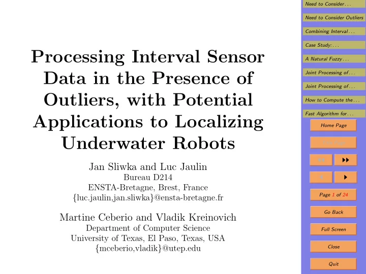
Need to Consider . . . Need to Consider Outliers Combining Interval . . . Case Study: . . . Processing Interval Sensor A Natural Fuzzy . . . Data in the Presence of Joint Processing of . . . Joint Processing of . . . Outliers, with Potential How to Compute the . . . Fast Algorithm for . . . Applications to Localizing Home Page Underwater Robots Title Page ◭◭ ◮◮ Jan Sliwka and Luc Jaulin Bureau D214 ◭ ◮ ENSTA-Bretagne, Brest, France Page 1 of 24 { luc.jaulin,jan.sliwka } @ensta-bretagne.fr Go Back Martine Ceberio and Vladik Kreinovich Department of Computer Science Full Screen University of Texas, El Paso, Texas, USA { mceberio,vladik } @utep.edu Close Quit
Need to Consider . . . Need to Consider Outliers 1. Need to Consider Interval Uncertainty Combining Interval . . . • The value � x measured by a sensor is, in general, differ- Case Study: . . . ent from the actual (unknown) value x . A Natural Fuzzy . . . Joint Processing of . . . • Traditionally, in science and engineering, it is assumed Joint Processing of . . . that we know the probability distribution of How to Compute the . . . def ∆ x = � x − x. Fast Algorithm for . . . Home Page • However, in many real-life situations, we only know the Title Page upper bound ∆ on the measurement error: | ∆ x | ≤ ∆. ◭◭ ◮◮ • In this case, the only information that we have about ◭ ◮ the actual value x is that x ∈ x = [ x, x ], where Page 2 of 24 x = � x − ∆ and x = � x + ∆ . Go Back • It is therefore important to consider interval uncer- Full Screen tainty. Close Quit
Need to Consider . . . Need to Consider Outliers 2. Need to Consider Outliers Combining Interval . . . • These exist many efficient techniques for processing Case Study: . . . such interval data. A Natural Fuzzy . . . Joint Processing of . . . • These techniques form an important part of granular Joint Processing of . . . computing . How to Compute the . . . • In practice, sensor malfunction sometimes produces Fast Algorithm for . . . outliers , values outside the interval [ � x − ∆ , � x + ∆]. Home Page • Outliers are usually characterized by a proportion ε of Title Page measurement results that could be erroneous. ◭◭ ◮◮ • For example, ε = 0 . 1 means that at least α = 1 − ε = ◭ ◮ 90% of the intervals contain the actual values. Page 3 of 24 • Sometimes, we do not know ε , so we should produce Go Back results corresponding to different values ε . Full Screen Close Quit
Need to Consider . . . Need to Consider Outliers 3. Combining Interval Uncertainty and Outliers: Combining Interval . . . What is Known Case Study: . . . • In general, outliers turn easy-to-solve interval problems A Natural Fuzzy . . . into difficult-to-solve (NP-hard) ones. Joint Processing of . . . Joint Processing of . . . • This is true even in the simplest case, when we simply repeatedly measure several quantities x 1 , . . . , x d . How to Compute the . . . Fast Algorithm for . . . • After each measurement, we get a box Home Page X ( j ) = [ x j ) 1 , x ( j ) 1 ] × . . . × [ x ( j ) d , x ( j ) d ] . Title Page • In the absence of outliers, the actual state belongs to ◭◭ ◮◮ the easy-to-compute intersection of all these boxes. ◭ ◮ • With outliers, the problem becomes NP-hard :-( Page 4 of 24 • For fixed d , there is a polynomial-time algorithm for Go Back solving this problem; its running time is O ( n d ). Full Screen • However, this running time grows exponentially with the dimension d . Close Quit
Need to Consider . . . Need to Consider Outliers 4. Case Study: Localizing Underwater Robots Combining Interval . . . • For underwater robot localization, we use distance mea- Case Study: . . . surements produced by sonars. A Natural Fuzzy . . . Joint Processing of . . . • A sonar measures echoes from the desired object and Joint Processing of . . . from other objects along the path. How to Compute the . . . • Example: a robot tries to localize itself by measuring Fast Algorithm for . . . the distance to the nearest wall. Home Page • Problem: the sensor may detect a reflection from the Title Page surface wave, a fish or a diver – producing an outlier. ◭◭ ◮◮ • After several measurements, we get a significant num- ◭ ◮ ber of outliers. Page 5 of 24 Go Back Full Screen Close Quit
Need to Consider . . . Need to Consider Outliers 5. Efficient Algorithm for the Simplest Situation Combining Interval . . . • We have n interval measurements [ x ( j ) , x ( j ) ] of the same Case Study: . . . quantity x . A Natural Fuzzy . . . Joint Processing of . . . • We know the upper bound ε > 0 on the proportion of Joint Processing of . . . measurements which are outliers. How to Compute the . . . • This means that the actual (unknown) value x satisfies at least n · (1 − ε ) of n constraints x ( j ) ≤ x ≤ x ( j ) . Fast Algorithm for . . . Home Page • To find the set of all such x , we sort all the endpoints Title Page x ( j ) and x ( j ) into a sequence x (1) ≤ x (2) ≤ . . . ≤ x (2 n ) . ◭◭ ◮◮ • This divides the set of possible values of x into 2 n − 1 ◭ ◮ zones [ x (1) , x (2) ], [ x (2) , x (3) ], . . . , [ x (2 n − 1) , x (2 n ) ]. Page 6 of 24 • For each zone k , we count the number of constraints c k which are satisfied for elements of this zone. Go Back • If c k ≥ n · (1 − ε ), we add k -th zone to the desired set. Full Screen • This takes time O ( n · log( n )) + O ( n ) = O ( n · log( n )). Close Quit
Need to Consider . . . Need to Consider Outliers 6. What if we Are Only Interested in the Interval Combining Interval . . . of Possible Values Case Study: . . . • Example: A Natural Fuzzy . . . Joint Processing of . . . – as a result of measuring the same quantity, we get Joint Processing of . . . two intervals [ − 2 , − 1] and [1 , 2]; How to Compute the . . . – since their intersection is empty, we know that one Fast Algorithm for . . . of them is an outlier; Home Page – let us assume that we know that one of them is Title Page correct. ◭◭ ◮◮ • In this case, the set of all possible values of x is the set ◭ ◮ [ − 2 , − 1] ∪ [1 , 2]. Page 7 of 24 • In this situation, the smallest possible value of x is − 2, and the largest possible value of x is 2. Go Back • Thus, the smallest interval that contains all possible Full Screen values of x is the interval [ − 2 , 2]. Close Quit
Need to Consider . . . Need to Consider Outliers 7. Computing Interval of Possible Values: Analy- Combining Interval . . . sis of the Problem and the Resulting Algorithm Case Study: . . . • Let us sort all n upper endpoints x ( j ) , 1 ≤ j ≤ n , into A Natural Fuzzy . . . an increasing sequence u 1 ≤ u 2 ≤ . . . ≤ u n . Joint Processing of . . . Joint Processing of . . . • We can guarantee that x is smaller than or equal to at How to Compute the . . . least n · (1 − ε ) terms in this sequence; so, x i ≤ u n · ε . Fast Algorithm for . . . • Similarly, if we sort x ( j ) , 1 ≤ j ≤ n , into ℓ 1 ≤ ℓ 2 ≤ Home Page . . . ≤ ℓ n , then we conclude that x ≥ ℓ n · (1 − ε ) . Title Page • Thus, we can conclude that the desired interval of pos- ◭◭ ◮◮ sible values x is equal to [ ℓ n · (1 − ε ) , u n · ε ]. ◭ ◮ • Finding elements of a given rank can be done in linear Page 8 of 24 time O ( n ). Go Back • Our preliminary experiments confirm that this tech- nique correctly locates the underwater robot. Full Screen Close Quit
Need to Consider . . . Need to Consider Outliers 8. A Natural Fuzzy Representation of Our Prob- Combining Interval . . . lem Case Study: . . . • For each x , we can find the proportion µ ( x ) ∈ [0 , 1] of A Natural Fuzzy . . . constraints which are satisfied for this x . Joint Processing of . . . Joint Processing of . . . • It is reasonable to interpret the resulting function µ ( x ) How to Compute the . . . as a membership function. Fast Algorithm for . . . • The actual value x must belong to the set of all the Home Page values x for which µ ( x ) ≥ 1 − ε . Title Page • Thus, the set of all possible x is the α -cut, with ◭◭ ◮◮ α = 1 − ε. ◭ ◮ • Up to now, fuzzy sets are just an interpretation. Page 9 of 24 • We will see that by using known fuzzy algorithms, we Go Back can speed up computations. Full Screen • Thus, fuzzy interpretation is indeed helpful. Close Quit
Recommend
More recommend
Explore More Topics
Stay informed with curated content and fresh updates.
