Probabilistic Partial Evaluation: Exploiting rule structure in - PowerPoint PPT Presentation

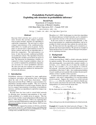
Probabilistic Partial Evaluation: Exploiting rule structure in probabilistic inference David Poole University of British Columbia 1

Overview • Belief Networks • Variable Elimination Algorithm • Parent Contexts & Structured Representations • Structure-preserving inference • Conclusion 2

Belief (Bayesian) Networks n � P ( x 1 , . . . , x n ) = P ( x i | x i − 1 . . . x 1 ) i = 1 n � = P ( x i | π x i ) i = 1 π x i are parents of x i : set of variables such that the predecessors are independent of x i given its parents. 3

Variable Elimination Algorithm Given: Bayesian Network, Query variable, Observations, Elimination ordering on remaining variables 1. set observed variables 2. sum out variables according to elimination ordering 3. renormalize 4

Summing Out a Variable ... h ... ... ... ... c g e f d a b ... ... Sum out e :  P ( a | c , d , e )    P ( a , b | c , d , f , g , h ) P ( b | e , f , g )   P ( e | h )  5

Structured Probability Tables P ( b | e , f , g ) P ( a | c , d , e ) d f t f g e e c t t f f p 1 p 2 p 3 p 4 p 5 p 6 p 7 p 8 p 2 = P ( a = t | d = t ∧ e = f ) 6

Eliminating e , preserving structure • We only need to consider a & b together when d = true ∧ f = true . In this context c & g are irrelevant. • In all other contexts we can consider a & b separately. • When d = false ∧ f = false , e is irrelevant. In this context the probabilities shouldn’t be affected by eliminating e . 7

Contextual Independence Given a set of variables C , a context on C is an assignment of one value to each variable in C . Suppose X , Y and C are disjoint sets of variables. X and Y are contextually independent given context c ∈ val ( C ) if P ( X | Y = y 1 ∧ C = c ) = P ( X | Y = y 2 ∧ C = c ) for all y 1 , y 2 ∈ val ( Y ) such that P ( y 1 ∧ c ) > 0 and P ( y 2 ∧ c ) > 0. 8

Parent Contexts A parent context for variable x i is a context c for a subset of the predecessors for x i such that x i is contextually independent of the other predecessors given c . For variable x i & assignment x i − 1 = v i − 1 , . . . , x 1 = v 1 of values to its preceding variables, there is a parent context π v i − 1 ... v 1 . x i P ( x 1 = v 1 , . . . , x n = v n ) n � = P ( x i = v n | x i − 1 = v i − 1 , . . . , x 1 = v 1 ) i = 1 n P ( x i = v i | π v i − 1 ... v 1 � = ) x i i = 1 9

Idea behind probabilistic partial evaluation • Maintain “rules” that are statements of probabilities in contexts. • When eliminating a variable, you can ignore all rules that don’t involve that variable. • This wins when a variable is only in few parent contexts. • Eliminating a variable looks like resolution! 10

Rule-based representation of our example a ← d ∧ e : p 1 b ← f ∧ e : p 5 a ← d ∧ e : p 2 b ← f ∧ e : p 6 a ← d ∧ c : p 3 b ← f ∧ g : p 7 a ← b ∧ c : p 4 b ← f ∧ g : p 8 e ← h : p 9 e ← h : p 10 11

Eliminating e a ← d ∧ e : p 1 b ← f ∧ e : p 5 a ← d ∧ e : p 2 b ← f ∧ e : p 6 a ← d ∧ c : p 3 b ← f ∧ g : p 7 a ← b ∧ c : p 4 b ← f ∧ g : p 8 e ← h : p 9 e ← h : p 10 unaffected by eliminating e 12

Variable partial evaluation If we are eliminating e , and have rules: x ← y ∧ e : p 1 x ← y ∧ e : p 2 e ← z : p 3 • no other rules compatible with y contain e in the body • y & z are compatible contexts, we create the rule: x ← y ∧ z : p 1 p 3 + p 2 ( 1 − p 3 ) 13

Splitting Rules A rule a ← b : p 1 can be split on variable d , forming rules: a ← b ∧ d : p 1 a ← b ∧ d : p 1 14

Why Split? If there are different contexts for a given e and for a given e , you need to split the contexts to make them directly comparable: � a ← b ∧ c ∧ e : p 1 a ← b ∧ e : p 1 a ← b ∧ c ∧ e : p 1 a ← b ∧ c ∧ e : p 2 a ← b ∧ c ∧ e : p 3 15

Combining Heads Rules a ← c : p 1 b ← c : p 2 where a and b refer to different variables, can be combined producing: a ∧ b ← c : p 1 p 2 Thus in the context with a , b , and c all true, the latter rule can be used instead of the first two. 16

Splitting Compatible Bodies a ← d ∧ e : p 1 b ← f ∧ e : p 5 a ← d ∧ f ∧ e : p 1 b ← d ∧ f ∧ e : p 5 a ← d ∧ f ∧ e : p 1 b ← d ∧ f ∧ e : p 5 a ← d ∧ e : p 2 b ← f ∧ e : p 6 a ← d ∧ f ∧ e : p 2 b ← d ∧ f ∧ e : p 6 a ← d ∧ f ∧ e : p 2 b ← d ∧ f ∧ e : p 6 e ← h : p 9 e ← h : p 10 17

Combining Rules a ← d ∧ f ∧ e : p 1 b ← d ∧ f ∧ e : p 5 a ← d ∧ f ∧ e : p 1 b ← d ∧ f ∧ e : p 5 a ← d ∧ f ∧ e : p 2 b ← d ∧ f ∧ e : p 6 a ← d ∧ f ∧ e : p 2 b ← d ∧ f ∧ e : p 6 e ← h : p 9 e ← h : p 10 18

Result of eliminating e The resultant rules encode the probabilities of { a , b } in the contexts: d ∧ f ∧ h , d ∧ f ∧ h For all other contexts we consider a and b separately. The resulting number of rules is 24. Tree structured probability for P ( a , b | c , d , f , g , h , i ) has 72 leaves. (Same as number of rules if a and b are combined in all contexts). VE has a table of size 256. 19

Evidence We can set the values of all evidence variables before summing out the remaining non-query variables. Suppose e 1 = o 1 ∧ . . . ∧ e s = o s is observed: • Remove any rule that contains e i = o ′ i , where o i �= o ′ i in the body. • Remove any term e i = o i in the body of a rule. • Replace any e i = o ′ i , where o i �= o ′ i , in the head of a rule false . • Replace any e i = o i in the head of a rule by true . In rule heads, use true ∧ a ≡ a , and false ∧ a ≡ false . 20

Conclusions • New notion of parent context � ⇒ rule-based representation for Bayesian networks. • New algorithm for probabilistic inference that preserves rule-structure. • Exploits more structure than tree-based representations of conditional probability. • Allows for finer-grained approximation than in a Bayesian network. 21