Probabilistic Foundations of Statistical Network Analysis Chapter 5: - PowerPoint PPT Presentation

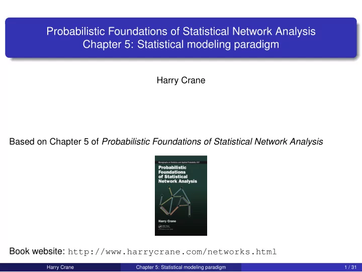
Probabilistic Foundations of Statistical Network Analysis Chapter 5: Statistical modeling paradigm Harry Crane Based on Chapter 5 of Probabilistic Foundations of Statistical Network Analysis Book website: http://www.harrycrane.com/networks.html Harry Crane Chapter 5: Statistical modeling paradigm 1 / 31

Table of Contents Chapter 1 Orientation 2 Binary relational data 3 Network sampling 4 Generative models 5 Statistical modeling paradigm 6 Vertex exchangeability 7 Getting beyond graphons 8 Relative exchangeability 9 Edge exchangeability 10 Relational exchangeability 11 Dynamic network models Harry Crane Chapter 5: Statistical modeling paradigm 2 / 31

Chapters 3 and 4 highlight two primary contexts of network analysis: Chapter 3: modeling sampled network data. Chapter 4: modeling evolving networks. Immediate observations: The concept of ‘network’ should not be conflated with the mathematical notion of ‘graph’ (Chapter 1). Sampling mechanism plays important role in model specification and statistical inference from sampled networks (Chapter 3). Statistical units are determined by the way in which the data is observed (Section 3.7). The explicit and implicit units should be aligned so that model-based inferences are compatible with their intended interpretation (Section 3.8). In this chapter, think of Y N as generic ‘network data’ of ‘size’ N in space N N of all such networks, where the interpretation of ‘network’ depends on context and ‘size’ is the number of units in that context. In Section 2.4, N N = { 0 , 1 } N × N and the size is the number of vertices. In Section 3.6.1.1, N N is the set of edge-labeled graphs with N edges and size is the number of edges. In Section 3.6.1.3, N N is the set of path-labeled graphs with N paths and size is the number of paths. Harry Crane Chapter 5: Statistical modeling paradigm 3 / 31

What is a statistical model? According to conventional wisdom in statistics literature: A statistical model is a set of probability distributions on the sample space. Questions : Just a set: { P 1 , P 2 , . . . } ? Harry Crane Chapter 5: Statistical modeling paradigm 4 / 31

All models are wrong ... All models are wrong, but some are useful. George Box (1919–2013) A statistical model is a set of probability distributions on the sample space. Questions : How can a set be ‘wrong’? What determines whether this set is ‘useful’? Harry Crane Chapter 5: Statistical modeling paradigm 5 / 31

Summary of Conclusions (I) What is a statistical model? Model = Description + Context ‘set’ + ‘inference rules’ (II) All models are wrong, but some are useful. First step to being ‘useful’ is ‘making sense’. Coherence : Model and inferences ‘make sense’ in a single context. (III) Network Modeling : Sound theory for network analysis should be built on models that are (i) coherent and (ii) account for realistic sampling schemes. Harry Crane Chapter 5: Statistical modeling paradigm 6 / 31

Role of the model All models are wrong, but some are useful. A statistical model is a set of probability distributions on the sample space. Role of the model in statistics : Sometimes exploratory data analysis (EDA) More often inference (out of sample) and prediction Asymptotic approximations When is a model useful for these purposes? Harry Crane Chapter 5: Statistical modeling paradigm 7 / 31

Just one set? Scenario : X 1 , X 2 , . . . are i.i.d. N ( µ, 1 ) . Observe : X ∗ 1 , . . . , X ∗ n for some finite n ≥ 1. Model : Set of distributions {N ( µ, 1 ) : −∞ < µ < ∞} on R . What can I do with this? Estimate population parameter µ based on sample X ∗ 1 , . . . , X ∗ n . (e.g., MLE, Bayesian posterior inference, ...) What makes this possible? Assumed: X 1 , X 2 , . . . i.i.d. N ( µ, 1 ) (population data). Implicit: X ∗ 1 , . . . , X ∗ n i.i.d. N ( µ, 1 ) (sampled data). Relationship between population and sample left implicit by convention. Leaving relationship between inferential universe (population) and observed data (sample) ambiguous causes confusion in more complicated situations. Harry Crane Chapter 5: Statistical modeling paradigm 8 / 31

Modeling household sizes Scenario : X 1 , . . . , X N are sizes (i.e., # of residents) of N households in a population. Household sizes are i.i.d. from a ‘1-shifted Poisson’: Pr ( X i = k + 1 ; λ ) = λ k e − λ / k ! , k = 0 , 1 , . . . . (1) Observe : X ∗ 1 , . . . , X ∗ n for some n < N . Model : (Depends on context) 1. X ∗ 1 , . . . , X ∗ n obtained by sampling uniformly without replacement from X 1 , . . . , X N . (Sampling households) X ∗ 1 , . . . , X ∗ = ⇒ i.i.d. from (1) . n 2. X ∗ 1 , . . . , X ∗ n obtained by sampling individuals in population and recording the size of their household. (Size-biased sampling) i = k + 1 ; λ ) = ( k + 1 ) λ k e − λ Pr ( X ∗ , k = 0 , 1 , . . . . ( λ + 1 ) k ! Harry Crane Chapter 5: Statistical modeling paradigm 9 / 31

What is a statistical model? A statistical model consists of M Description of the observed data: Set of candidate distributions C Context under which data observed: Relations among different sets For each n ≥ 1, the model ( M , C ) induces a set of candidate distributions M n for sample of size n . What makes a model M “statistical” is that it can be used for statistical inference. Requires the context C under which the inference is performed. Population Observed network (sample) Y N Y n M M n (induced by context) Model Harry Crane Chapter 5: Statistical modeling paradigm 10 / 31

What is a statistical model? A statistical model consists of M Description of the observed data: Set of candidate distributions C Context under which data observed: Relations among different sets For each n ≥ 1, the model ( M , C ) induces a set of candidate distributions M n for sample of size n . What makes a model M “statistical” is that it can be used for statistical inference. Requires the context C under which the inference performed. Example (i.i.d. sequence): M = {N ( µ, 1 ) : −∞ < µ < ∞} For n ≥ 1, ( X ∗ 1 , . . . , X ∗ n ) modeled as M n = {N ⊗ n ( µ, 1 ) : −∞ < µ < ∞} Example (household sizes): M = { 1-shifted Poisson ( λ ) : λ > 0 } For n ≥ 1, ( X ∗ 1 , . . . , X ∗ n ) modeled from size-biased distribution (assuming 2nd context of sampling individuals) Harry Crane Chapter 5: Statistical modeling paradigm 11 / 31

‘Using’ the model Given: model ( M , C ) with induced sample models {M n } n ≥ 1 . Given data D of size n ≥ 1. 1 Find optimal candidate distribution ˆ P n in M n based on D (according to some 2 criteria). Infer optimal distribution ˆ P M by interpreting ˆ P n in context C . 3 Example (i.i.d. sequence): M = {N ( µ, 1 ) : −∞ < µ < ∞} For n ≥ 1, ( X ∗ 1 , . . . , X ∗ n ) modeled as M n = {N ⊗ n ( µ, 1 ) : −∞ < µ < ∞} . Given ˆ µ, 1 ) infer ˆ P n = N ⊗ n (ˆ P M = N (ˆ µ, 1 ) . Example (household sizes): M = { 1-shifted Poisson ( λ ) : λ > 0 } For n ≥ 1, ( X ∗ 1 , . . . , X ∗ n ) modeled from size-biased distribution (assuming 2nd context of sampling individuals). Given ˆ P n from size-based with parameter ˆ λ n , infer population parameter through relationship ˆ λ n ↔ ˆ λ n − 1. Harry Crane Chapter 5: Statistical modeling paradigm 12 / 31

Sampling context (Example) For m ≤ n define selection sampling S m , n : R n → R m ( x 1 , . . . , x n ) �→ ( x 1 , . . . , x m ) For a distribution F on R n , let S m , n F denote distribution of S m , n X n for X n ∼ F . (Note: S m , n F = F S − 1 m , n , usual induced distribution) Given set M n , we write set of all induced distributions as S m , n M n = { S m , n F : F ∈ M n } . Population Observed network (sample) X X n ( X 1 , X 2 , . . . ) S n , N X = ( X 1 , . . . , X n ) S n , N M = M n = {N ⊗ n ( µ, 1 ) } M = {N ⊗∞ ( µ, 1 ) } Model Sampling scheme S m , n necessary to establish relationship between observation and population. Sampling mechanism often (almost always) left out of model specification. Harry Crane Chapter 5: Statistical modeling paradigm 13 / 31

General sampling context m , n : R n → R m by For m ≤ n and injection ψ : [ m ] → [ n ] , define ψ -sampling S ψ m , n : R n → R m S ψ ( x 1 , . . . , x n ) �→ ( x ψ ( 1 ) , . . . , x ψ ( m ) ) . Let Σ m , n be random sampling map obtained by choosing ψ : [ m ] → [ n ] randomly and putting Σ m , n = S ψ m , n . (Distribution of ψ can depend on X n .) Write Σ m , n F to denote the distribution of S ψ m , n X n for this randomly chosen ψ and X n ∼ F . Also write Σ m , n M n = { Σ m , n F : F ∈ M n } . Definition (Coherence) A statistical model ( {M n } n ≥ 1 , { Σ m , n } n ≥ m ≥ 1 ) is coherent if Σ m , n M n = M m for all n ≥ m ≥ 1 induced = specified Harry Crane Chapter 5: Statistical modeling paradigm 14 / 31

Coherent = ⇒ ‘useful’ Definition (Coherence) A statistical model ( {M n } n ≥ 1 , { Σ m , n } n ≥ m ≥ 1 ) is coherent if Σ m , n M n = M m for all n ≥ m ≥ 1 . Suppose ( {M n } n ≥ 1 , { Σ m , n } n ≥ m ≥ 1 ) is coherent. Given data D of size m ≥ 1. Estimate ˆ P m from M m given D . For n ≥ m , infer P n = { F ∈ M n : Σ m , n F = ˆ ˆ P m } . * This set is a singleton if model is identifiable. For smaller sample size ( ℓ ≤ m ) estimate P ℓ = Σ ℓ, m ˆ ˆ P m . Coherence needed to guarantee (i) ˆ P n is non-empty and (ii) ˆ P ℓ ∈ M ℓ . Harry Crane Chapter 5: Statistical modeling paradigm 15 / 31