Privacy preserving data mining randomized response and association - PowerPoint PPT Presentation
Privacy preserving data mining randomized response and association rule hiding Li Xiong CS573 Data Privacy and Anonymity Partial slides credit: W. Du, Syracuse University, Y. Gao, Peking University Privacy Preserving Data Mining
Privacy preserving data mining – randomized response and association rule hiding Li Xiong CS573 Data Privacy and Anonymity Partial slides credit: W. Du, Syracuse University, Y. Gao, Peking University
Privacy Preserving Data Mining Techniques Protecting sensitive raw data Randomization (additive noise) Geometric perturbation and projection (multiplicative noise) Randomized response technique Categorical data perturbation in data collection model Protecting sensitive knowledge (knowledge hiding)
Data Collection Model Data cannot be shared directly because of privacy concern
Background: Randomized Response The true Do you smoke? answer is “Yes” Yes Head Biased coin: P ( Yes ) P ( Head ) ( 0 . 5 ) No 0 . 5 Tail P '( Yes ) P ( Yes ) P ( No ) (1 ) P '( No ) P ( Yes ) (1 ) P ( No )
Decision Tree Mining using Randomized Response Multiple attributes encoded in bits True answer E: 110 Head Biased coin: P ( Yes ) P ( Head ) ( 0 . 5 ) Tail False answer !E: 001 0 . 5 Column distribution can be estimated for learning a decision tree! Using Randomized Response Techniques for Privacy-Preserving Data Mining, Du, 2003
Accuracy of Decision tree built on randomized response
Generalization for Multi-Valued Categorical Data S i q1 S i+1 q2 q3 S i+2 q4 True Value: S i S i+3 P '( s 1) q 1 q 4 q 3 q 2 P ( s 1) M P '( s 2) q 2 q 1 q 4 q 3 P ( s 2) P '( s 3) q 3 q 2 q 1 q 4 P ( s 3) P '( s 4) q 4 q 3 q 2 q 1 P ( s 4)
A Generalization RR Matrices [Warner 65], [R.Agrawal 05], [S. Agrawal 05] RR Matrix can be arbitrary a 11 a 12 a 13 a 14 a 21 a 22 a 23 a 24 M a 31 a 32 a 33 a 34 a 41 a 42 a 43 a 44 Can we find optimal RR matrices? OptRR:Optimizing Randomized Response Schemes for Privacy-Preserving Data Mining, Huang, 2008
What is an optimal matrix? Which of the following is better? 1 0 0 1 1 1 3 3 3 M 1 M 2 1 1 1 0 1 0 3 3 3 1 1 1 0 0 1 3 3 3 Privacy: M 2 is better Utility: M 1 is better So, what is an optimal matrix?
Optimal RR Matrix An RR matrix M is optimal if no other RR matrix’s privacy and utility are both better than M (i, e, no other matrix dominates M). Privacy Quantification Utility Quantification A number of privacy and utility metrics have been proposed. Privacy: how accurately one can estimate individual info. Utility: how accurately we can estimate aggregate info.
Metrics Privacy: accuracy of estimate of individual values Utility: difference between the original probability and the estimated probability
Optimization Methods Approach 1: Weighted sum: w 1 Privacy + w 2 Utility Approach 2 Fix Privacy, find M with the optimal Utility. Fix Utility, find M with the optimal Privacy. Challenge: Difficult to generate M with a fixed privacy or utility. Proposed Approach: Multi-Objective Optimization
Optimization algorithm Evolutionary Multi-Objective Optimization (EMOO) The algorithm Start with a set of initial RR matrices Repeat the following steps in each iteration Mating : selecting two RR matrices in the pool Crossover : exchanging several columns between the two RR matrices Mutation : change some values in a RR matrix Meet the privacy bound : filtering the resultant matrices Evaluate the fitness value for the new RR matrices. Note : the fitness values is defined in terms of privacy and utility metrics
Illustration
Output of Optimization The optimal set is often plotted in the objective space as Pareto front . Worse M 6 M 5 M 4 M 8 M 7 M 3 M 1 M 2 Utility Better Privacy
For First attribute of Adult data
Privacy Preserving Data Mining Techniques Protecting sensitive raw data Randomization (additive noise) Geometric perturbation and projection (multiplicative noise) Randomized response technique Protecting sensitive knowledge (knowledge hiding) Frequent itemset and association rule hiding Downgrading classifier effectiveness
Frequent Itemset Mining and Association Rule Mining Frequent itemset mining: frequent set of items in a transaction data set Association rules: associations between items
Frequent Itemset Mining and Association Rule Mining First proposed by Agrawal, Imielinski, and Swami in SIGMOD 1993 SIGMOD Test of Time Award 2003 “This paper started a field of research. In addition to containing an innovative algorithm, its subject matter brought data mining to the attention of the database community … even led several years ago to an IBM commercial, featuring supermodels, that touted the importance of work such as that contained in this paper. ” Apriori algorithm in VLDB 1994 #4 in the top 10 data mining algorithms in ICDM 2006 R. Agrawal, T. Imielinski, and A. Swami. Mining association rules between sets of items in large databases. In SIGMOD ’93. Apriori: Rakesh Agrawal and Ramakrishnan Srikant. Fast Algorithms for Mining Association Rules. In VLDB '94.
Basic Concepts: Frequent Patterns and Association Rules Itemset: X = {x 1 , …, x k } (k-itemset) Transaction-id I tems bought Frequent itemset: X with minimum 10 A, B, D support count 20 A, C, D Support count (absolute support): count 30 A, D, E of transactions containing X 40 B, E, F Association rule: A B with minimum 50 B, C, D, E, F support and confidence Support: probability that a transaction Customer Customer contains A B buys both buys diaper s = P(A B) Confidence: conditional probability that a transaction having A also contains B c = P(A | B) Association rule mining process Customer Find all frequent patterns (more costly) buys beer February 19, 2009 Generate strong association rules 20
Illustration of Frequent Itemsets and Association Rules Transaction-id I tems bought 10 A, B, D 20 A, C, D 30 A, D, E 40 B, E, F 50 B, C, D, E, F Frequent itemsets (minimum support count = 3) ? { A:3, B:3, D:4, E:3, AD:3} Association rules (minimum support = 50%, minimum confidence = 50%) ? A D (60%, 100%) D A (60%, 75%) February 19, 2009
Association Rule Hiding: what? why?? Problem : hide sensitive association rules in data without losing non-sensitive rules Motivations : confidential rules may have serious adverse effects SIGMOD Ph.D. Workshop 22 IDAR ’ 07
Problem statement Given a database D to be released minimum threshold “ MST ” , “ MCT ” a set of association rules R mined from D a set of sensitive rules R h R to be hided Find a new database D ’ such that the rules in R h cannot be mined from D ’ the rules in R-R h can still be mined as many as possible SIGMOD Ph.D. Workshop IDAR ’ 07
Solutions Data modification approaches Basic idea: data sanitization D -> D ’ Approaches: distortion,blocking Drawbacks Cannot control hiding effects intuitively, lots of I/O Data reconstruction approaches Basic idea: knowledge sanitization D -> K -> D ’ Potential advantages Can easily control the availability of rules and control the hiding effects directly, intuitively, handily SIGMOD Ph.D. Workshop IDAR ’ 07
Distortion-based Techniques Sample Database Distorted Database Sample Database Distorted Database A B C D A B C D Distortion 1 1 1 0 1 1 1 0 Algorithm 1 0 1 1 1 0 0 1 0 0 0 0 1 0 0 0 1 1 1 1 0 1 1 1 0 1 0 1 1 1 0 0 1 0 Rule A → → C has: Rule A → → C has now: Rule A Rule A C has: C has now: → C → C A → A → Support(A C)= 80% )= 80% Support(A C)= 40% )= 40% Support( Support( → C → C A → A → Confidence(A C)= 100% )= 100% Confidence(A C)= 50% )= 50% Confidence( Confidence(
Side Effects Before Hiding Before Hiding After Hiding After Hiding Side Effect Side Effect Process Process Process Process Rule R i has had Rule R i has now Rule Eliminated conf(R i conf(R i )< MCT )< MCT conf(R i )> MCT (Undesirable Side conf(R i )> MCT Effect) Rule R i has had Rule R i has now Ghost Rule conf(R i )> MCT conf(R i )> MCT conf(R i )< MCT (Undesirable Side conf(R i )< MCT Effect) Large Itemset I has Itemset I has now Itemset Eliminated had sup(I sup(I )> MST )> MST sup(I )< MST )< MST sup(I (Undesirable Side Effect)
Distortion-based Techniques Challenges/Goals: To minimize the undesirable Side Effects that the hiding process causes to non-sensitive rules. To minimize the number of 1 1’ ’s s that must be deleted in the database. Algorithms must be linear in time as the database increases in size.
Sensitive itemsets: ABC
Recommend
More recommend
Explore More Topics
Stay informed with curated content and fresh updates.

