Practical Interpretation With a quantitative factor, like power in - PowerPoint PPT Presentation

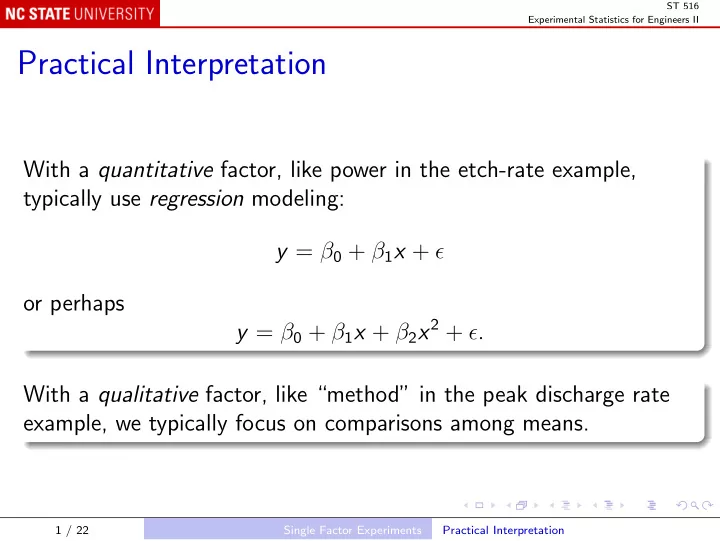
ST 516 Experimental Statistics for Engineers II Practical Interpretation With a quantitative factor, like power in the etch-rate example, typically use regression modeling: y = β 0 + β 1 x + ǫ or perhaps y = β 0 + β 1 x + β 2 x 2 + ǫ. With a qualitative factor, like “method” in the peak discharge rate example, we typically focus on comparisons among means. 1 / 22 Single Factor Experiments Practical Interpretation

ST 516 Experimental Statistics for Engineers II Comparing Means A contrast is a linear combination of treatment means: a a � � c i µ i , with c i = 0 . i =1 i =1 Examples are: µ 1 − µ 2 , where c 1 = 1 , c 2 = − 1 , c 3 = ... = c a = 0; µ 1 − 1 2 ( µ 2 + µ 3 ), where c 1 = 1 , c 2 = c 3 = − 1 2 , c 4 = ... = c a = 0. 2 / 22 Single Factor Experiments Practical Interpretation

ST 516 Experimental Statistics for Engineers II Testing a Contrast Many hypotheses about treatment means can be written in terms of a contrast: a � H 0 : c i µ i = 0 i =1 for appropriate contrast constants c 1 , c 2 , . . . , c a . We estimate � a i =1 c i µ i by a a � � c i ˆ µ i = c i ¯ y i · = C . i =1 i =1 3 / 22 Single Factor Experiments Practical Interpretation

ST 516 Experimental Statistics for Engineers II C is an unbiased estimator, with a V ( C ) = σ 2 � c 2 i , n i =1 which we estimate by a V ( C ) = MS E ˆ � c 2 i . n i =1 The test statistic is therefore a � c i ¯ y i · C i =1 t 0 = = . � � ˆ MS E � a i =1 c 2 V ( C ) n i 4 / 22 Single Factor Experiments Practical Interpretation

ST 516 Experimental Statistics for Engineers II Compare t 0 with the t -distribution with df = N − a . Equivalently, compare F 0 = t 2 0 with the F -distribution with df = 1 , N − a . Confidence interval for C : � a a � � MS E � � � c 2 c i ¯ y i · ± t α/ 2 , N − a i . n i =1 i =1 5 / 22 Single Factor Experiments Practical Interpretation

ST 516 Experimental Statistics for Engineers II Multiple Contrasts Sometimes we test several contrasts in the same experiment, or equivalently set up CIs for those contrasts; error rate becomes an issue. Control experiment-wise error rate for all possible contrasts using � Scheff´ e’s method: replace t α/ 2 , N − a with ( a − 1) F α, a − 1 , N − a . Confidence interval becomes � a a � � MS E � � � � c 2 c i ¯ y i · ± ( a − 1) F α, a − 1 , N − a i . n i =1 i =1 6 / 22 Single Factor Experiments Practical Interpretation

ST 516 Experimental Statistics for Engineers II Pairwise Comparisons Often the only contrasts we consider are pairwise comparisons µ i − µ j . To control experiment-wise error rate for all pairwise comparisons , Tukey’s method gives shorter intervals than Scheff´ e’s: CI is � MS E y i · − ¯ ¯ y j · ± q α ( a , f ) , n where q α ( a , f ) is a percent point of the studentized range statistic, and f = N − a is the degrees of freedom in MS E . 7 / 22 Single Factor Experiments Practical Interpretation

ST 516 Experimental Statistics for Engineers II Fisher’s Least Significant Difference The basic t -statistic for comparing µ i with µ j is y i · − ¯ ¯ y j · t 0 = � . � � n i + 1 1 MS E n j So we declare µ i and µ j to be significantly different if � 1 � + 1 � | ¯ y i · − ¯ y j · | > t α/ 2 , N − a MS E . n i n j 8 / 22 Single Factor Experiments Practical Interpretation

ST 516 Experimental Statistics for Engineers II That is, � 1 � + 1 � MS E t α/ 2 , N − a n i n j is the least significant difference , or LSD. Notes In a balanced design, n i = n j = n , so the LSD is the same for every pair µ i and µ j . The LSD method has comparison-wise error rate α ; it does not control experimentwise error rate. 9 / 22 Single Factor Experiments Practical Interpretation

ST 516 Experimental Statistics for Engineers II R command TukeyHSD(aov(EtchRate ~ factor(Power), etchRateLong)) Output Tukey multiple comparisons of means 95% family-wise confidence level Fit: aov(formula = EtchRate ~ factor(Power), data = etchRateLong) $‘factor(Power)‘ diff lwr upr p adj 180-160 36.2 3.145624 69.25438 0.0294279 200-160 74.2 41.145624 107.25438 0.0000455 220-160 155.8 122.745624 188.85438 0.0000000 200-180 38.0 4.945624 71.05438 0.0215995 220-180 119.6 86.545624 152.65438 0.0000001 220-200 81.6 48.545624 114.65438 0.0000146 10 / 22 Single Factor Experiments Practical Interpretation

ST 516 Experimental Statistics for Engineers II Graph plot(TukeyHSD(aov(EtchRate ~ factor(Power), etchRateLong))) 95% family−wise confidence level 180−160 200−160 220−160 200−180 220−180 220−200 0 50 100 150 Differences in mean levels of factor(Power) 11 / 22 Single Factor Experiments Practical Interpretation

ST 516 Experimental Statistics for Engineers II Sample Size Using Operating Characteristic curves: β is the probability of type II error: β = 1 − P { Reject H 0 | H 0 is false } = 1 − P { F 0 > F α, a − 1 , N − a | H 0 is false } . Charts plot β against Φ, where Φ 2 = n � a i =1 τ 2 i . a σ 2 So if we know σ 2 and a set of treatment effects τ 1 , τ 2 , . . . , τ a for which we want the type II error to be β , we can find the smallest acceptable n . 12 / 22 Single Factor Experiments Sample Size

ST 516 Experimental Statistics for Engineers II Note: often the resulting n is too large for the experiment to be feasible. The experimenter must accept higher β or larger τ ’s. Alternative to using OC charts: using length of confidence interval; for comparing two means, confidence interval is � MS E × 2 y i · − ¯ ¯ y j · ± t α/ 2 , N − a n , If we know σ 2 , can choose n to give desired width. Still often gives infeasible (too large) n . 13 / 22 Single Factor Experiments Sample Size

ST 516 Experimental Statistics for Engineers II The Regression Approach Recall the “effects” model: y i , j = µ + τ i + ǫ i , j , i = 1 , 2 , . . . , a , j = 1 , 2 , . . . , n i . Note that we now allow for unbalanced data (unequal n i ). 14 / 22 Single Factor Experiments The Regression Approach

ST 516 Experimental Statistics for Engineers II Suppose we put all the y ’s in a response vector :   y 1 , 1 y 1 , 2   .   .  .      y 1 , n 1     y 2 , 1     y 2 , 2   .   . Y = .     y 2 , n 2     . .   .     y a , 1     y a , 2     . .   .   y a , n a 15 / 22 Single Factor Experiments The Regression Approach

ST 516 Experimental Statistics for Engineers II To keep track of the group that an observation belongs to, we also create a design matrix X . The row for an observation in group i consists of all zeroes, except for a single 1 at position i . For convenience, we add a first column with all 1’s. 16 / 22 Single Factor Experiments The Regression Approach

ST 516 Experimental Statistics for Engineers II   1 1 0 . . . 0 1 1 0 0 . . .   . . . . .   . . . . .  . . . . .     1 1 0 . . . 0     1 0 1 0  . . .     1 0 1 . . . 0   . . . . .   . . . . . X = . . . . .     1 0 1 0 . . .     . . . . . . . . . .   . . . . .     1 0 0 1 . . .     1 0 0 . . . 1    . . . . .  . . . . .   . . . . .   1 0 0 1 . . . 17 / 22 Single Factor Experiments The Regression Approach

ST 516 Experimental Statistics for Engineers II We also put all the parameters µ, τ 1 , τ 2 , . . . , τ a into a parameter vector :   µ τ 1     τ 2 β =   .   .  .    τ a With an error vector ǫ constructed like Y , we have Y = X β + ǫ . 18 / 22 Single Factor Experiments The Regression Approach

ST 516 Experimental Statistics for Engineers II This is a multiple regression equation. The least squares estimates ˆ µ, ˆ τ 1 , ˆ τ 2 , . . . , ˆ τ a satisfy the least squares normal equations X ′ X ˆ β = X ′ Y . If X ′ X were non-singular, we could solve these equations: ˆ β = ( X ′ X ) − 1 X ′ Y . But it isn’t, so we can’t... 19 / 22 Single Factor Experiments The Regression Approach

ST 516 Experimental Statistics for Engineers II The first column of X is the sum of the other columns, which makes one column redundant. More formally, if   +1 − 1     − 1 b = ,   .   .  .    − 1 then ( X ′ X ) b = X ′ ( Xb ) = 0 . So X ′ X is singular. 20 / 22 Single Factor Experiments The Regression Approach

ST 516 Experimental Statistics for Engineers II If we leave out one column of X , the remaining columns have no redundancy, and the reduced X ′ X matrix is non-singular. Leaving out a column means leaving the corresponding parameter out of the model. Leave out the first column ⇔ leave out µ ⇔ the means model. Leave out the second column ⇔ leave out τ 1 ⇔ the effects model with the first level as the baseline. Leave out the last column ⇔ leave out τ a ⇔ the effects model with the last level as the baseline. 21 / 22 Single Factor Experiments The Regression Approach