Power k -Means Clustering (Poster #96) Jason Xu and Kenneth Lange - PowerPoint PPT Presentation
Power k -Means Clustering (Poster #96) Jason Xu and Kenneth Lange Department of Statistical Science, Duke University Departments of Biomathematics, Statistics, Human Genetics, UCLA Thirty-sixth International Conference on Machine
Power k -Means Clustering (Poster #96) Jason Xu ‡ and Kenneth Lange ∗ ‡ Department of Statistical Science, Duke University ∗ Departments of Biomathematics, Statistics, Human Genetics, UCLA Thirty-sixth International Conference on Machine Learning June 13, 2019, Long Beach, CA 1
Partitional clustering and k -means • Given a representation of n observations and a measure of similarity, seek an optimal partition C = { C 1 , . . . , C k } into k groups • X ∈ R d × n denotes n datapoints, θ ∈ R d × k represent k centers • k -means: assign each observation to the cluster represented by the nearest center, minimizing within-cluster variance k k � � � � x − θ j � 2 argmin = argmin | C j | Var ( C j ) C C j =1 x ∈ C j j =1 2
Lloyd’s algorithm (1957) Greedy approach: seeks local minimizer of k -means objective, rewritten n � 1 ≤ j ≤ k � x i − θ j � 2 := f −∞ ( θ ) min i =1 1. Update label assignments: C ( m ) = { x i : θ ( m ) is closest center } j j 1 � 2. Recompute centers by averaging: θ ( m +1) = x i j | C ( m ) | j x i ∈ C ( m ) j Simple yet effective, remains most widely used clustering algorithm 3
Issues even when implicit assumptions are met 4
Drawbacks of Lloyd’s algorithm Even in ideal settings, Lloyd’s algorithm is prone to local minima • Sensitive to initialization, gets trapped in poor solutions, worsens in high dimensions • Objective is non-smooth, highly non-convex • “External” improvements: good initialization schemes ( k -means++) Goal: an “internal” improvement that retains the simplicity of Lloyd’s algorithm, and seeks to optimize the same measure of quality Solution: annealing along a continuum of smooth surfaces via majorization-minimization 5
A geometric approach: k -harmonic means (2001) � � − 1 � k 1 j =1 x − 1 H ( x 1 , . . . , x k ) = as a proxy for min( x 1 , . . . , x k ) k j Zhang et al. propose instead minimizing the criterion n k � 1 � � � x i − θ j � − 2 � − 1 := f − 1 ( θ ) k i =1 j =1 6
A member of the power means family � 1 � s for z i ∈ (0 , ∞ ) � k 1 i =1 z s Class of power means : M s ( z ) = i k • s = 1 yields arithmetic mean, s = − 1 yields harmonic mean, etc • Continuous, symmetric, homogeneous, strictly increasing • Will be useful to generalize the good intuition behind KHM Classical mathematical results ⇒ nice algorithmic properties 1. Well-known s →−∞ M s ( z 1 , . . . , z k ) = min { z 1 , . . . , z k } lim 2. Power mean inequality M s ( z 1 , . . . , z k ) ≤ M t ( z 1 , . . . , z k ) , s ≤ t 7
From power means to clustering criteria � 1 � � k s 1 i =1 z s Recall M s ( z ) = k i n k � 1 � � � x i − θ j � − 2 � − 1 f − 1 ( θ ) = (KHM) k i =1 j =1 • substitute z j = � x i − θ j � 2 into M − 1 ( z ), sum over i n � 1 ≤ j ≤ k � x i − θ j � 2 f −∞ ( θ ) = min ( k -means) i =1 • the same, substituting instead into “ M −∞ ( z )” What about all the other power means? 8
A continuum of smoother objectives Figure: A cross-section of the k -means objective − f −∞ ( θ ) with k = 3 clusters in dimension d = 1. Third center is fixed at its true value. 9
A continuum of smoother objectives (b) s = − 1 . 0 (KHM) (a) s = − 10 . 0 9
A continuum of smoother objectives (c) s = − 0 . 2 (d) s = 0 . 3 9
Gradually approaching the k -means criterion For any { s ( m ) } → −∞ , lim Proposition: m →∞ min θ f s ( m ) ( θ ) = min θ f −∞ ( θ ) . • Choosing one instance (i.e. f − 1 ) as proxy may not always be a good idea, now interpreted as early stopping along solution path • Starting at s (0) < 1, gradually decreasing s → −∞ can be understood as a form of annealing 10
Toward an iterative solution: majorization-minimization A surrogate g ( θ | θ m ) is said to majorize the function f ( θ ) at θ m if f ( θ m ) = g ( θ m | θ m ) tangency at θ m f ( θ ) ≤ g ( θ | θ m ) domination for all θ . MM algorithm: iterates θ m +1 = argmin g ( θ | θ n ) θ • Example: Expectation-Maximization (EM) is an example of MM • Lloyd’s algorithm can be considered EM for Gaussian mixtures with limiting σ 2 → 0 11
Illustration of MM algorithm larger f(x) smaller very bad optimal less bad x 12
Illustration of MM algorithm larger ● f(x) smaller very bad optimal less bad x 12
Illustration of MM algorithm larger ● f(x) smaller very bad optimal less bad x 12
Illustration of MM algorithm larger ● ● f(x) smaller very bad optimal less bad x 12
Illustration of MM algorithm larger ● ● ● f(x) smaller very bad optimal less bad x 12
Illustration of MM algorithm larger ● ● ● f(x) smaller very bad optimal less bad x 12
Illustration of MM algorithm larger ● ● ● f(x) ● ● smaller very bad optimal less bad x 12
Illustration of MM algorithm larger ● ● ● f(x) ● ● smaller ● ● ● very bad optimal less bad x 12
Illustration of MM algorithm larger ● ● ● f(x) ● ● smaller ● ●● ● ● ● ● very bad optimal less bad x 12
By all means, k -means · Same O ( nkd ) time complexity as Lloyd; one additional parameter s (0) For any decreasing sequence s ( m ) ≤ 1 , the iterates θ ( m ) Proposition: produced by Algorithm 1 generates a decreasing sequence of objective values f s ( m ) ( θ ( m ) ) bounded below by 0. As a consequence, the sequence of objective values converges. 13
The shape of power means to come � 1 k � 1 s − 1 1 ∂ � z s k z s − 1 Gradient has a nice form: ∂ z j M s ( z 1 , . . . , z k ) = i j k i =1 Quadratic form of Hessian (not shown) shows that M s ( z ) is concave for s ≤ 1 This means that whenever s ≤ 1, the following inequality holds: k ∂ M s ( z ( m ) , . . . , z ( m ) � ∂ z j M s ( z ( m ) , . . . , z ( m ) )( z j − z ( m ) M s ( z 1 , . . . , z k ) ≤ ) + ) 1 k 1 k j j =1 14
Minimizing power means objectives Let w ( m ) ∂ θ j M s ( � x i − θ ( m ) � 2 , . . . , � x i − θ ( m ) � 2 ) for a given value θ ( m ) ∂ = 1 ij k C ( m ) � �� � n n k � � � � � w ( m ) � x i − θ ( m ) M s ( θ ( m ) ; x i ) + f s ( θ ) = M s ( θ ; x i ) ≤ � j ij i =1 i =1 j =1 + � n � k � x i − θ j � 2 := g ( θ | θ ( m ) ) j =1 w ( m ) i =1 ij Unlike objective f s ( θ ), the right-hand side g ( θ | θ ( m ) ) is easy to minimize! n n 1 � � w ( m ) w ( m ) ˆ 0 = − 2 ( x i − θ j ) , θ j = x i . ij � n ij i =1 w ( m ) i =1 ij i =1 15
Analogous experiment in KHM paper when d = 2 16
Performance comparison Table: Variation of information under k -means++ initialization d = 2 d = 5 d = 10 d = 20 d = 50 d = 100 d = 200 Lloyd 0.637 0.261 0.234 0.223 0.199 0.206 0.183 KHM 0.651 0.328 0.339 0.319 0.263 0.280 0.231 s 0 =-1 ( 0.593) ( 0.199) 0.133 0.136 0.084 0.087 0.069 − 3 0.593 0.226 ( 0.111) ( 0.069) ( 0.022) ( 0.027) 0.026 − 9 0.608 0.252 0.199 0.169 0.078 0.036 ( 0.026) − 18 0.615 0.259 0.218 0.208 0.140 0.101 0.077 Power k -means performs best for all choices of s (0) under good seedings! 17
Performance comparison Table: Root k -means quality ratio with k -means++ initialization d = 2 d = 5 d = 10 d = 20 d = 50 d = 100 d = 200 Lloyd 1.036 1.236 1.363 1.411 1.476 1.492 1.481 KHM 1.044 1.290 1.473 1.504 1.556 1.586 1.556 s 0 =-1 ( 1.029) ( 1.164) 1.185 1.221 1.178 1.181 1.149 − 3 1.030 1.187 ( 1.155) ( 1.110) ( 1.044) ( 1.054) ( 1.059) − 9 1.032 1.220 1.293 1.296 1.192 1.086 1.069 − 18 1.034 1.228 1.328 1.370 1.351 1.254 1.203 Other measures such as adjusted Rand index convey the same trends 18
Closing remarks • KHM degrades rapidly as d increases, and its benefits become less noticeable even in the plane with the availability of good seedings • Power k -means succeeds in settings where Lloyd’s and KHM break down, despite “ideal” setting • Speed: power k -means takes ≈ 50 iterations ( ≈ 20 seconds) on MNIST with n = 60 000 , d = 784 • Convergence rates ⇒ optimal annealing schedules, choices of s (0) ? • Bregman and other non-Euclidean extensions 19
Thank you! Poster #96 jason.q.xu@duke.edu // jasonxu90.github.io 20
Recommend
More recommend
Explore More Topics
Stay informed with curated content and fresh updates.


