Population sizing Correct size of the population important: too - PowerPoint PPT Presentation
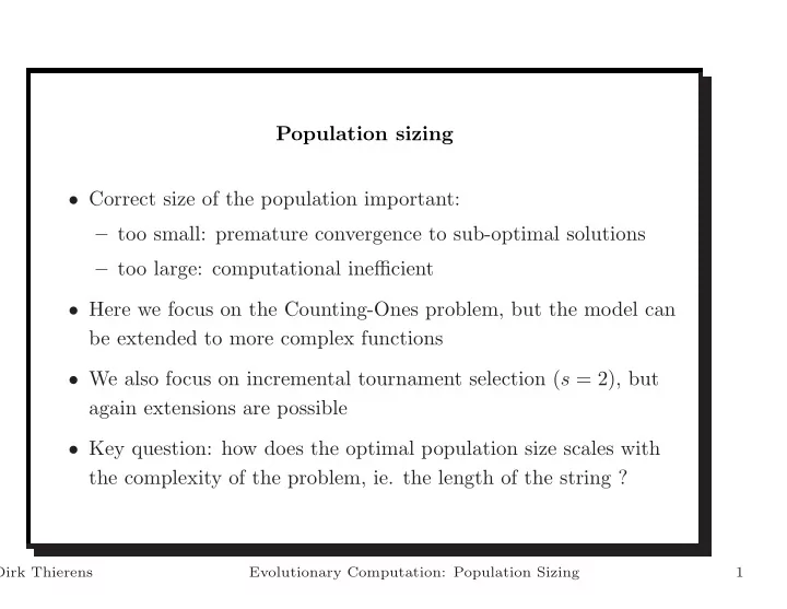
Population sizing Correct size of the population important: too small: premature convergence to sub-optimal solutions too large: computational inefficient Here we focus on the Counting-Ones problem, but the model can be extended to
Population sizing • Correct size of the population important: – too small: premature convergence to sub-optimal solutions – too large: computational inefficient • Here we focus on the Counting-Ones problem, but the model can be extended to more complex functions • We also focus on incremental tournament selection ( s = 2), but again extensions are possible • Key question: how does the optimal population size scales with the complexity of the problem, ie. the length of the string ? Dirk Thierens Evolutionary Computation: Population Sizing 1
Selection error • Tournament selection ( s = 2): two strings compete to become member of the parent pool: s 1 : 1100011100, fitness = 5 s 2 : 0100111101, fitness = 6 string s 2 is selected • Looking at this competition at the schema level (order-1 sufficient since we focus one Counting-Ones): – partition f ∗ ∗ ∗ ∗ ∗ ∗ ∗ ∗∗ : schema 0 ∗ ∗ ∗ ∗ ∗ ∗ ∗ ∗∗ wins from schema 1 ∗ ∗ ∗ ∗ ∗ ∗ ∗ ∗∗ ⇒ selection decision error – partitions ∗ ∗ ∗ ∗ f ∗ ∗ ∗ ∗∗ and ∗ ∗ ∗ ∗ ∗ ∗ ∗ ∗ ∗ f : schema ∗ ∗ ∗ ∗ 1 ∗ ∗ ∗ ∗∗ wins from schema ∗ ∗ ∗ ∗ 0 ∗ ∗ ∗ ∗ , and schema ∗ ∗ ∗ ∗ ∗ ∗ ∗ ∗ ∗ 1 wins from schema ∗ ∗ ∗ ∗ ∗ ∗ ∗ ∗ 0 ⇒ correct selection decisions Dirk Thierens Evolutionary Computation: Population Sizing 2
– other partitions: nothing changes • How many selection decision errors can we afford to make before the optimal bit-value within a partition is completely lost in the population = premature convergence • Population sizing is basically a statistical decision making problem Dirk Thierens Evolutionary Computation: Population Sizing 3
Binomial distribution • Random variable X is binomial distributed if it has the discrete probability density: x ∈ { 0 , . . . , ℓ } � ℓ p x (1 − p ) ℓ − x � f ( x ) = P ( X = x ) = x • The probability distribution function corresponding to the binomial density is: x � � ℓ p p (1 − p ) ℓ − k � F X ( x ) = P ( X ≤ x ) = k k =0 mean: µ = ℓp variance: σ 2 = ℓp (1 − p ) Dirk Thierens Evolutionary Computation: Population Sizing 4
Normal distribution • Random variable X is normal distributed if it has the discrete probability density: x ∈ ℜ 1 2 ( x − µ ) 2 e − 1 √ f ( x ) = σ 2 πσ • The probability distribution function corresponding to the normal density is (mean µ , variance σ 2 ): � x 1 2 ( y − µ ) 2 dy e − 1 √ F X ( x ) = σ 2 πσ −∞ • Standard normal variable: X ∼ N (0 , 1) � x 1 e − y 2 2 dy Φ( z ) = F Z ( z ) = √ 2 π −∞ and P ( a ≤ Z ≤ b ) = Φ( b ) − Φ( a ) Dirk Thierens Evolutionary Computation: Population Sizing 5
Normal approximation to the binomial distribution • Assume random variable X ℓ is binomial distributed with parameters ℓ and p . If ℓ → ∞ the probability distribution function of the standardized X ℓ − ℓp √ random variable X ∗ ℓ = ℓp (1 − p ) approaches the probability distribution function Φ of the standard normal distribution: x − ℓp x − ℓp P ( X ∗ ℓ ≤ ) ≈ Φ( ) � � ℓp (1 − p ) ℓp (1 − p ) or x − ℓp P ( X ℓ ≤ x ) ≈ Φ( ) � ℓp (1 − p ) The approximation is acceptable when minimum( ℓp, ℓ (1 − p )) ≥ 5 b − ℓp a − ℓp √ √ • note: p ( a ≤ X ℓ ≤ b ) ≈ Φ( ℓp (1 − p ) ) − Φ( ℓp (1 − p ) ) Dirk Thierens Evolutionary Computation: Population Sizing 6
Probability selection decision error • Schemata fitness f ( H 1 : ∗ ∗ ∗ 1 ∗ ∗ ∗ ∗ ∗ ∗ ∗ ∗ ) and f ( H 2 : ∗ ∗ ∗ 0 ∗ ∗ ∗ ∗ ∗ ∗ ∗ ∗ ) binomial distributed → approximating with normal distribution N ( µ, σ 2 ): σ 2 µ H 1 = 1 + ( ℓ − 1) p, H 1 = ( ℓ − 1) p (1 − p ) σ 2 µ H 2 = ( ℓ − 1) p, H 2 = ( ℓ − 1) p (1 − p ) • Distribution of the fitness difference of the best schema and the worst schema f ( H 1 ) − f ( H 2 ) is also normal distributed: σ 2 µ H 1 − H 2 = 1 , H 1 − H 2 = 2( ℓ − 1) p (1 − p ) • Probability selection error is equal to the probability that the best schema is represented by a string with fitness less than the representative of the worst schema, which is also equal to the Dirk Thierens Evolutionary Computation: Population Sizing 7
probability that the fitness difference is negative: P [ SelErr ] = P ( F H 1 − H 2 < 0) P ( F H 1 − H 2 − µ H 1 − H 2 < − µ H 1 − H 2 = ) σ H 1 − H 2 σ H 1 − H 2 − 1 = Φ( ) � 2( ℓ − 1) p (1 − p ) 0.5 0.45 0.4 0.35 probability selection error 0.3 0.25 0.2 l=400 l=200 l=100 l= 50 0.15 0.1 0.05 0 0.5 0.55 0.6 0.65 0.7 0.75 0.8 0.85 0.9 0.95 1 proportion p bit values 1 Dirk Thierens Evolutionary Computation: Population Sizing 8
• Approximation by first two terms of power series expansion for the normal distribution: 1 1 P [ SelErr ] ≈ 2 − � 2 π ( ℓ − 1) p (1 − p ) 0.5 0.45 0.4 0.35 probability selection error 0.3 0.25 0.2 l=400 l=200 l=100 l= 50 0.15 0.1 0.05 0 0.5 0.55 0.6 0.65 0.7 0.75 0.8 0.85 0.9 0.95 1 proportion bit values 1 Dirk Thierens Evolutionary Computation: Population Sizing 9
• Selection error is upper bounded by: P [ SelErr ] ≤ 1 1 2 − √ , πℓ this is a conservative estimate of the selection error that ignores the reduction in error probability when the proportion of optimal bit values p ( t ) increases. 0.5 0.45 0.4 0.35 probability selection error 0.3 0.25 0.2 P[SelErr] Upper Bound P[SelErr] 0.15 0.1 0.05 0 0.5 0.55 0.6 0.65 0.7 0.75 0.8 0.85 0.9 0.95 1 proportion bit values 1 Dirk Thierens Evolutionary Computation: Population Sizing 10
GA population sizing • Selection viewed as decision making process within partitions: schemata competition • When best schema looses competition we have a selection decision error • How many decision errors can we afford to make given a certain population size ? • Answer given by Gambler’s ruin model: within each partition a random walk is played Dirk Thierens Evolutionary Computation: Population Sizing 11
Random walks Random walks are mathematical models used to predict the outcome of certain stochastic processes. Consider the following random walk: 1. a one-dimensional, discrete space of size N + 1: [0 , 1 , . . . , N − 1 , N ] 2. a particle somewhere in the above space: position x ∈ { 0 , . . . , N } 3. the particle can move one step to the right with probability p , and one step to the left with probability 1 − p 4. when the particle reaches the boundaries ( x = 0, or x = N ) the random walk ends 5. call P N ( x ) (resp. P 0 ( x )) the probability that the particle is absorbed by the boundary x = N (resp, x = 0) when it is currently at position x Dirk Thierens Evolutionary Computation: Population Sizing 12
• Difference equation: P N ( x ) = pP N ( x + 1) + (1 − p ) P N ( x − 1) with boundary conditions: P N ( N ) = 1, and P N (0) = 0 • Solving the above equation gives the probability that the particle - starting from position x 0 - is absorbed by the x = N boundary: 1 − ( 1 − p p ) x 0 P N ( x 0 ) = 1 − ( 1 − p p ) N • when p = 1 − p = 0 . 5 we get P N ( x 0 ) = x 0 N note also: P 0 ( x 0 ) = 1 − P N ( x 0 ) Dirk Thierens Evolutionary Computation: Population Sizing 13
Gambler’s ruin model The previous random walk is called the Gambler’s ruin model describing a gambler betting against a casino: 1. the position x represents the amount of money a gambler possesses 2. the size N represents the total amount of money of the gambler and the casino 3. p (resp. 1 − p ) is the probability the gambler wins (resp. looses) a bet, and he subsequently gains (resp. looses) one unit of money 4. P 0 ( x 0 ) (resp. P N ( x 0 )) is the probability the gambler is ruined (resp. breaks the casino) when starting with x 0 amount of money Dirk Thierens Evolutionary Computation: Population Sizing 14
Population sizing & Gambler’s ruin Mapping GA concepts in Gambler’s ruin model: 1. The number of optimal bit values ’1’ in the population at a certain position - this is, for the partition considered - corresponds to the position x in the Gambler’s ruin model 2. The boundaries x = N (resp. x = 0) correspond to all bit values in the population at the partition being equal to the bit value ’1’ (resp, ’0’) 3. When the boundaries are reached the random walk ends: either the population is filled with ones at the partition or filled with zeroes (recall that we do not take mutation into account here) 4. The probability that the amount of optimal string values in the population at the partition is increased by one is equal to the Dirk Thierens Evolutionary Computation: Population Sizing 15
probability that the selection decision making is correct for that partition. This corresponds to the probability that the particle moves to the right ( p ) 5. Desired convergence corresponds to the particle reaching the x = N boundary. Premature convergence - this is, loosing the optimal bit value in the population - corresponds to the particle reaching the x = 0 boundary. Recalling the probability for a selection decision error (using tournament selection, s = 2): P [ SelErr ] ≤ 1 1 2 − √ πℓ we can compute the probability of convergence to the optimal bit Dirk Thierens Evolutionary Computation: Population Sizing 16
Recommend
More recommend
Explore More Topics
Stay informed with curated content and fresh updates.
