Pipeline for Our Example Using SCALE Atmel dataset A Acquire - PowerPoint PPT Presentation

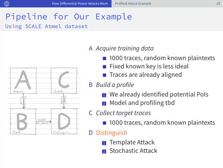
How Differential Power Attacks Work Profiled Attack Example 28 Pipeline for Our Example Using SCALE Atmel dataset A Acquire training data 1000 traces, random known plaintexts Fixed known key is less ideal Traces are already aligned B Build a profile 1 We already identified potential PoIs 2 Model and profiling tbd C Collect target traces 1000 traces, random known plaintexts D Distinguish 1 Template Attack 2 Stochastic Attack

How Differential Power Attacks Work Profiled Attack Example 29 Template Attacks Naive Bayes i x i power k 0 score 0 12 1.35... 0 0.134... 1 123 4.65... 1 0.116... . . . . . . ⇒ . . . . . . . . . . . . . . . . . . 255 0.098... 999 59 2.79... 1. From Probability to Likelihood For each key candidate k determine its a posteriori probability given the observed leakage L

How Differential Power Attacks Work Profiled Attack Example 29 Template Attacks Naive Bayes i x i power k 0 score 0 12 1.35... 0 0.134... 1 123 4.65... 1 0.116... . . . . . . ⇒ . . . . . . . . . . . . . . . . . . 255 0.098... 999 59 2.79... 1. From Probability to Likelihood Pr[ k | L ] = Pr[ L | k ] · Pr[ k ] Pr[ L ] Pr[ L | k ] is the likelihood Pr[ k ] and Pr[ L ] can be ignored

How Differential Power Attacks Work Profiled Attack Example 29 Template Attacks Naive Bayes i x i power k 0 score 0 12 1.35... 0 0.134... 1 123 4.65... 1 0.116... . . . . . . ⇒ . . . . . . . . . . . . . . . . . . 255 0.098... 999 59 2.79... 2. From Likelihood to Sum of Log Likelihoods Assume each trace leaks independently, then � Pr[ L | k ] = Pr[ L i | k ] i

How Differential Power Attacks Work Profiled Attack Example 29 Template Attacks Naive Bayes i x i power k 0 score 0 12 1.35... 0 0.134... 1 123 4.65... 1 0.116... . . . . . . ⇒ . . . . . . . . . . . . . . . . . . 255 0.098... 999 59 2.79... 2. From Likelihood to Sum of Log Likelihoods Assume each trace leaks independently, then afer taking logs � log 2 Pr[ L | k ] = log 2 Pr[ L i | k ] i

How Differential Power Attacks Work Profiled Attack Example 29 Template Attacks Naive Bayes i x i power k 0 score 0 12 1.35... 0 0.134... 1 123 4.65... 1 0.116... . . . . . . ⇒ . . . . . . . . . . . . . . . . . . 255 0.098... 999 59 2.79... From Log Likelihood to QDA Assume L ( data ) ∼ ˆ M ( x i ⊕ k ∗ ) + N ( 0 , σ ) then log 2 Pr[ L i | k ] = log 2 N ( L i − ˆ M ( x i ⊕ k ); 0 , σ )

How Differential Power Attacks Work Profiled Attack Example 29 Template Attacks Naive Bayes i x i power score k 0 0 12 1.35... 0 0.134... 1 123 4.65... 1 0.116... . . . . . . ⇒ . . . . . . . . . . . . . . . . . . 255 0.098... 999 59 2.79... From Log Likelihood to QDA Assume L ( data ) ∼ ˆ M ( x i ⊕ k ∗ ) + N ( 0 , σ ) then � 2 / 2 σ 2 − 1 � L i − ˆ log 2 Pr[ L i | k ] = − log 2 e M ( x i ⊕ k ) 2 ( 1 + log 2 π ) − σ

How Differential Power Attacks Work Profiled Attack Example 29 Template Attacks Naive Bayes i x i power score k 0 0 12 1.35... 0 0.134... 1 123 4.65... 1 0.116... . . . . . . ⇒ . . . . . . . . . . . . . . . . . . 255 0.098... 999 59 2.79... QDA Summary � ( L i − ˆ M ( x i ⊕ k )) 2 score ( k | L ) = i To profile: ˆ M ( z ) for all 256 possible z Warning: Scores can no longer be interpreted as posteriors

How Differential Power Attacks Work Profiled Attack Example 30 Template and Stochastic Attacks SCALE Atmel Profiling 0.04 0.04 0.02 0.02 0.00 0.00 0.02 0.02 0.04 0.04 0 50 100 150 200 250 0 50 100 150 200 250 11005 11223 Template Attack For all 256 possible S-box input values determine the sample mean (optional) determine the sample variance Problem: 1000 traces is not enough to estimate 256 parameters

How Differential Power Attacks Work Profiled Attack Example 30 Template and Stochastic Attacks SCALE Atmel Profiling Original data Original data 0.04 0.04 Fitted line Fitted line 0.03 0.02 0.02 0.00 0.01 0.02 0.00 0.04 0.01 0 1 2 3 4 5 6 7 8 0 1 2 3 4 5 6 7 8 11005 11223 Stochastic Attack Assume the leakage model M a , b ( k , x ) = a · HammingWeight ( Sbox ( x ⊕ k )) + b estimate a and b ( Warning: The right estimation is naively unweighted)

How Differential Power Attacks Work Profiled Attack Example 31 Template Attacks SCALE Atmel Scores 7000 49000 6000 48000 5000 47000 4000 46000 3000 45000 2000 0 50 100 150 200 250 0 50 100 150 200 250 11005 11223 Final distinguishing scores Afer incorporating 1000 target traces left One candidate key very clearly sticks out right One candidate key sticks out, but not as much

How Differential Power Attacks Work Profiled Attack Example 31 Template Attacks SCALE Atmel Scores 10 60.0 57.5 8 55.0 52.5 6 50.0 4 47.5 45.0 2 42.5 0 40.0 0 200 400 600 800 1000 0 200 400 600 800 1000 11005 11223 Evolution of distinguishing scores Look at scores as a function of number of traces incorporated left the true key quickly separates from the rest right it takes much longer for the true key to stand out In blue the actual keybyte

How Differential Power Attacks Work Profiled Attack Example 31 Template Attacks SCALE Atmel Scores 175 14 150 12 125 10 100 8 75 6 50 4 25 2 0 0 0.0 2.5 5.0 7.5 10.0 12.5 15.0 17.5 0.0 2.5 5.0 7.5 10.0 12.5 15.0 17.5 11005 11223 Evolution of distinguishing scores Look at scores as a function of number of traces incorporated left the true key quickly separates from the rest right it takes much longer for the true key to stand out In blue the actual keybyte

How Differential Power Attacks Work Profiled Attack Example 32 Template Attacks SCALE Atmel Success Rate 0.25 0.8 0.20 0.6 0.15 0.4 0.10 0.2 0.05 0.0 0.00 0.0 2.5 5.0 7.5 10.0 12.5 15.0 17.5 0 25 50 75 100 125 150 175 200 11005 11223 Success Rate: Probability that best guess wins For each i (x-axis), ran 2000 experiments: 1 Selected i out of 1000 traces 2 Check if best guess is actual keybyte Warning: resampling methodology used due to available data

How Differential Power Attacks Work Profiled Attack Example 32 Template Attacks SCALE Atmel Success Rate 0.25 0.8 0.20 0.6 0.15 0.4 0.10 0.2 0.05 0.0 0.00 0.0 2.5 5.0 7.5 10.0 12.5 15.0 17.5 0 25 50 75 100 125 150 175 200 11005 11223 Success rate conclusion 1 Lef performs better than right 2 Success rate 2 − 2 for a single keybyte, only gives 2 − 32 for the full 16-byte key. Note: jaggedness likely due to low number of experiments

Key Enumeration and Ranking Enumeration 33 Different Adversarial Scenarios Not-Quite-Kerckhoffs Principle C ← E K ∗ ( X ) K ∗ ← $ Kg L ← $ Leak ( K ∗ , X ) L ← Leak ( K, X ) ❆ K win ← K = K ∗ win ˆ K The adversary can exhaustively search the key

Key Enumeration and Ranking Enumeration 33 Different Adversarial Scenarios Not-Quite-Kerckhoffs Principle C ← E K ∗ ( X ) K ∗ ← $ Kg L ← $ Leak ( K ∗ , X ) Leak ← $ L L X K , X L ← Leak ( K, X ) ❆ L K win ← K = K ∗ win ˆ K The adversary can enumerate the key

Key Enumeration and Ranking Enumeration 34 Enumeration Enhancing Divide-and-Conquer Attacks k 0 score k 1 score k 15 score 0 0.123... 0 0.134... 0 0.184... 1 0.127... 1 0.116... 1 0.167... ... . . . . . . . . . . . . . . . . . . 255 0.238... 255 0.098... 255 0.152... Best guess Simply output the most likely 128-bit key overall Key enumeration Test keys from most likely to least likely until success

Key Enumeration and Ranking Enumeration 34 Enumeration Enhancing Divide-and-Conquer Attacks k 0 score k 1 score k 15 score 0 0.123... 0 0.134... 0 0.184... 1 0.127... 1 0.116... 1 0.167... ... . . . . . . . . . . . . . . . . . . 255 0.238... 255 0.098... 255 0.152... Best guess obviously k 0 = 0, k 1 = 255, ..., k 15 = 255 But what about the next best guess? Question posed by Veyrat-Charvillon et al. (SAC’12)

Key Enumeration and Ranking Enumeration 34 Enumeration Enhancing Divide-and-Conquer Attacks k 0 score k 1 score k 15 score 0 0.123... 0 0.134... 0 0.184... 1 0.127... 1 0.116... 1 0.167... ... . . . . . . . . . . . . . . . . . . 255 0.238... 255 0.098... 255 0.152... DPA with Enumeration A number of cost metrics 1 The number of traces (profile vs.target) 2 The running time of the distinguisher 3 The number of keys to test 4 The overhead (in time) to enumerate

Key Enumeration and Ranking Enumeration 34 Enumeration Enhancing Divide-and-Conquer Attacks Some approaches Naive Create ordered list of all 2 128 keys 2012 Tree-like recursion algorithm [Veyrat-Charvillon, Gérard, Renauld, Standaert / SAC] 2015 Dynamic programming enabling parallellization [Martin, O’Connell, Oswald, Stam / Asiacrypt]

Key Enumeration and Ranking Enumeration 35 A Typical Side-Channel Attack Pipeline Adding Enumeration Afer the Distinguish phase, the scores are fed to an Enumeration phase

Key Enumeration and Ranking Enumeration 35 A Typical Side-Channel Attack Pipeline Adding Enumeration Afer the Distinguish phase, the scores are fed to an Enumeration phase But how long will it take, roughly? Question posed by Veyrat-Charvillon et al. (Eurocrypt’13)