Persistent homology of spaces and groups Graham Ellis Outline 1. - PowerPoint PPT Presentation
Persistent homology of spaces and groups Graham Ellis Outline 1. Introduction to persistence bar codes (three motivating examples) 2. Computation of persistence bar codes (discrete vector fields & contracting homotopies) 3. Potential
Persistent homology of spaces and groups Graham Ellis Outline 1. Introduction to persistence bar codes (three motivating examples) 2. Computation of persistence bar codes (discrete vector fields & contracting homotopies) 3. Potential application to group cohomology Mathematics Algorithms Proofs, 8-12 November 2010
Motivating Example I: statistical data analysis Given a set S of points randomly sampled from an unknown manifold M , what can we infer about the topology of M ?
Motivating Example I: statistical data analysis Given a set S of points randomly sampled from an unknown manifold M , what can we infer about the topology of M ? For instance, S sampled from M ⊂ R 2 .
One approach to data analysis Repeatedly “thicken” the set S to produce a sequence of inclusions S = S 1 ⊂ S 2 ⊂ S 3 ⊂ · · · . Then search for “persistent” topological features in the sequence. S
One approach to data analysis Repeatedly “thicken” the set S to produce a sequence of inclusions S = S 1 ⊂ S 2 ⊂ S 3 ⊂ · · · . Then search for “persistent” topological features in the sequence. S 3 S 4 S 2 S S 6 S 8 S 5 S 7
Betti numbers β 0 ( X ) = number of path components of X β 1 ( X ) = dim( H 1 ( X , Q ))
Betti numbers β 0 ( X ) = number of path components of X β 1 ( X ) = dim( H 1 ( X , Q )) S 1 S 2 S 3 S 4 S 5 S 6 S 7 S 8 β 0 478 32 9 2 1 1 1 1 β 1 115 19 These numbers are consistent with the sample coming from some region with the homotopy type of a circle.
Betti numbers β 0 ( X ) = number of path components of X β 1 ( X ) = dim( H 1 ( X , Q )) = number of 1-dimensional holes in X S 1 S 2 S 3 S 4 S 5 S 6 S 7 S 8 β 0 478 32 9 2 1 1 1 1 β 1 0 115 18 4 1 1 1 1
Betti numbers β 0 ( X ) = number of path components of X β 1 ( X ) = dim( H 1 ( X , Q )) = number of 1-dimensional holes in X S 1 S 2 S 3 S 4 S 5 S 6 S 7 S 8 β 0 478 32 9 2 1 1 1 1 β 1 0 115 18 4 1 1 1 1 These numbers are consistent with the sample coming from some region with the homotopy type of a circle.
During an inclusion S i ֒ → S j holes can ֒ → persist ֒ → die ֒ → be born
During an inclusion S i ֒ → S j holes can ֒ → persist ֒ → die ֒ → be born β ij n = number of n -dimensional holes in S i that persist to S j
During an inclusion S i ֒ → S j holes can ֒ → persist ֒ → die ֒ → be born β ij n = number of n -dimensional holes in S i that persist to S j β ij 0 = rank ( H n ( S i , Q ) − → H n ( S j , Q ))
Bar codes Matrix ( β ij n ) represented by graph with: ◮ vertices arranged in columns ◮ only horizontal edges ◮ i th column has β ii n = β n ( S i ) vertices ◮ β ij n paths from i th column to j th column
β 1 bar code for our example
β 0 bar code for our example (first column cropped)
D E F C A B G β 0 bar codes contain less information than dendrograms (or phylogenetic trees) A B C D E F G
How to thicken data? Low-dimensional data in R n : (digital images, dynamical systems, ...) Construct a filtered cubical subcomplex of R n . High-dimensional data: (statistical data sample of N points, ...) Construct a filtration on the simplex ∆ N . Group-theoretic data: Construct a filtration on a (regular CW) Eilenberg-MacLane space.
Motivating Example II: polymer growth How do the shapes of the following planar graphs differ?
Motivating Example II: polymer growth How do the shapes of the following planar graphs differ? MacPherson & Srolovitz: Persistent homology can capture shape.
Various thickenings of the first graph
β 1 bar code for first graph
β 1 bar code for second graph
MacPherson & Srolovitz define the “homological dimension” of a graph in terms of: ◮ The number of bars in its bar code ◮ the length of these bars ◮ the centres of these bars
Motivating Example III: medical images Digital images f : M → R could be analyzed using bar codes.
Motivating Example III: medical images Digital images f : M → R could be analyzed using bar codes. Consider a torus M , height function f f r barcode 0 b0 b1 b1 b2 and filtration M r = f − 1 ([0 , r ]) .
Motivating Example III: medical images Digital images f : M → R could be analyzed using bar codes. Consider a torus M , height function f f r bar code β 0 β 1 β 1 β 2 0 and filtration M r = f − 1 ([0 , r ]) .
Motivating Example III: medical images Digital images f : M → R could be analyzed using bar codes. Consider a torus M , height function f f r bar code β 0 β 1 β 1 β 2 β 1 0 and filtration M r = f − 1 ([0 , r ]) .
To compute the homlogy of a space X we impose some cell structure, and consider ∂ 2 ∂ 1 · · · → C 2 ( X ) → C 1 ( X ) → C 0 ( X ) → 0 C n ( X ) = vector space, basis ↔ n -cells ∂ n induced by cell boundaries H n ( X ) = ker( ∂ n ) / image ( ∂ n +1 )
To compute the homlogy of a space X X we impose some cell structure,
To compute the homlogy of a space X X we impose some cell structure, and consider · · · → C 2 ( X ) ∂ 2 → C 1 ( X ) ∂ 1 → C 0 ( X ) → 0 ◮ C n ( X ) = vector space, basis ↔ n -cells ◮ ∂ n induced by cell boundaries ◮ H n ( X ) = ker( ∂ n ) / image ( ∂ n +1 )
Our cubical representation of the thickened planar graph X = has 45467 2-cells, 91531 edges and 46060 vertices. A naive computation of H 1 ( X , F ) = F 5 is slow.
Simple homotopy collapses can yield homotopy retracts Y ⊂ X .
Simple homotopy collapses can yield homotopy retracts Y ⊂ X . If X = Y ∪ e n and Y ∩ e n ≃ ∗ then X ≃ Y . X Y ≃
For cubical subspaces of low-dimensional R n the test Y ∩ e n ≃ ∗ can be performed quickly.
For cubical subspaces of low-dimensional R n the test Y ∩ e n ≃ ∗ can be performed quickly. For cubcial X ⊂ R 2 a cell e 2 can be deleted without changing homotopy type iff its neighbourhood is one of a storable list: etc.
For cubical subspaces of low-dimensional R n the test Y ∩ e n ≃ ∗ can be performed quickly. For cubcial X ⊂ R 2 a cell e 2 can be deleted without changing homotopy type iff its neighbourhood is one of a storable list: etc. etc. Many neighbourhoods not in list:
The retract ≃ has only 1717 vertices, 2342 edges and 621 faces.
The retract ≃ has only 1717 vertices, 2342 edges and 621 faces. The retract Y has contractible subspace Z ⊂ Y with 1713 vertices, 2329 edges and 617 faces.
The retract ≃ has only 1717 vertices, 2342 edges and 621 faces. The retract Y has contractible subspace Z ⊂ Y with 1713 vertices, 2329 edges and 617 faces. The computation H 1 ( X , Z ) ∼ = H 1 ( C ∗ ( Y ) / C ∗ ( Z )) = Z 5 takes a fraction of a second.
Contracting homotopies From a homotopy retract Y ⊂ X we often need ◮ the chain inclusion ι ∗ : C ∗ ( Y ) ֒ → C ∗ ( X ) ◮ its quasi-inverse φ ∗ : C ∗ ( X ) → C ∗ ( Y ) ◮ and a family of homomorphisms h n : C n ( X ) → C n +1 ( X ) ( n ≥ 0) satisfying ι n φ n − 1 = ∂ n +1 h n + h n − 1 ∂ n ( h − 1 = 0) .
Contracting homotopies From a homotopy retract Y ⊂ X we often need ◮ the chain inclusion ι ∗ : C ∗ ( Y ) ֒ → C ∗ ( X ) ◮ its quasi-inverse φ ∗ : C ∗ ( X ) → C ∗ ( Y ) ◮ and a family of homomorphisms h n : C n ( X ) → C n +1 ( X ) ( n ≥ 0) satisfying ι n φ n − 1 = ∂ n +1 h n + h n − 1 ∂ n ( h − 1 = 0) . Discrete Morse Theory is handy for computing h n , φ n .
A discrete vector field on a regular CW-space X is a collection of arrows s → t where ◮ s , t are cells and any cell is involved in at most one arrow ◮ dim( t ) = dim( s ) + 1 ◮ s lies in the boundary of t
A discrete vector field on a regular CW-space X is a collection of arrows s → t where ◮ s , t are cells and any cell is involved in at most one arrow ◮ dim( t ) = dim( s ) + 1 ◮ s lies in the boundary of t ≃
A discrete vector field on a cellular space X is a collection of arrows s → t where ◮ s , t are cells and any cell is involved in at most one arrow ◮ dim( t ) = dim( s ) + 1 ◮ s lies in the boundary of t ≃
Continued example ≃
Continued example ≃ Theorem: If X is a regular CW-space with discrete vector field then there is a homotopy equivalence X ≃ Y where Y is a CW-space whose cells correspond to those of X not involved in any arrow.
Contracting homotopy Given a discrete vector field we define the contracting homotopy h n : C n ( X ) → C n +1 ( X ) on generators e n by if e n is not a source 0 � e n +1 ∂ n +1 ( � e n +1 h n ( e n ) = ) contains just the one i i source e n of dimension n
1 ) h 1 (e e 1
Group (co)homology Definition: The (co)homology of a group G is the (co)homology of X / G where X is any contractible space admitting a free G -action.
Group (co)homology Definition: The (co)homology of a group G is the (co)homology of X / G where X is any contractible space admitting a free G -action. Theorem: A CW-space X is contractible if π n ( X n +1 ) = 0 for n ≥ 0.
Recommend
More recommend
Explore More Topics
Stay informed with curated content and fresh updates.
