Part-II Parametric Signal Modeling and Linear Prediction Theory 2. - PowerPoint PPT Presentation

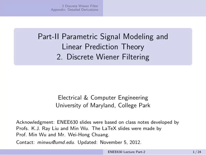
2 Discrete Wiener Filter Appendix: Detailed Derivations Part-II Parametric Signal Modeling and Linear Prediction Theory 2. Discrete Wiener Filtering Electrical & Computer Engineering University of Maryland, College Park Acknowledgment: ENEE630 slides were based on class notes developed by Profs. K.J. Ray Liu and Min Wu. The LaTeX slides were made by Prof. Min Wu and Mr. Wei-Hong Chuang. Contact: minwu@umd.edu . Updated: November 5, 2012. ENEE630 Lecture Part-2 1 / 24

2.0 Preliminaries 2 Discrete Wiener Filter 2.1 Background Appendix: Detailed Derivations 2.2 FIR Wiener Filter for w.s.s. Processes 2.3 Example Preliminaries [ Readings: Haykin’s 4th Ed. Chapter 2, Hayes Chapter 7 ] • Why prefer FIR filters over IIR? ⇒ FIR is inherently stable. • Why consider complex signals? Baseband representation is complex valued for narrow-band messages modulated at a carrier frequency. Corresponding filters are also in complex form. u [ n ] = u I [ n ] + ju Q [ n ] • u I [ n ]: in-phase component • u Q [ n ]: quadrature component the two parts can be amplitude modulated by cos 2 π f c t and sin 2 π f c t . ENEE630 Lecture Part-2 2 / 24

2.0 Preliminaries 2 Discrete Wiener Filter 2.1 Background Appendix: Detailed Derivations 2.2 FIR Wiener Filter for w.s.s. Processes 2.3 Example (1) General Problem (Ref: Hayes § 7.1) Want to process x [ n ] to minimize the difference between the estimate and the desired signal in some sense: A major class of estimation (for simplicity & analytic tractability) is to use linear combinations of x [ n ] (i.e. via linear filter). When x [ n ] and d [ n ] are from two w.s.s. random processes, we often choose to minimize the mean-square error as the performance index. � d [ n ] | 2 � � | e [ n ] | 2 � | d [ n ] − ˆ min w J � E = E ENEE630 Lecture Part-2 3 / 24

2.0 Preliminaries 2 Discrete Wiener Filter 2.1 Background Appendix: Detailed Derivations 2.2 FIR Wiener Filter for w.s.s. Processes 2.3 Example (2) Categories of Problems under the General Setup 1 Filtering 2 Smoothing 3 Prediction 4 Deconvolution ENEE630 Lecture Part-2 4 / 24

2.0 Preliminaries 2 Discrete Wiener Filter 2.1 Background Appendix: Detailed Derivations 2.2 FIR Wiener Filter for w.s.s. Processes 2.3 Example Wiener Problems: Filtering & Smoothing Filtering The classic problem considered by Wiener x [ n ] is a noisy version of d [ n ]: x [ n ] = d [ n ] + v [ n ] The goal is to estimate the true d [ n ] using a causal filter (i.e., from the current and post values of x [ n ]) The causal requirement allows for filtering on the fly Smoothing Similar to the filtering problem, except the filter is allowed to be non-causal (i.e., all the x [ n ] data is available) ENEE630 Lecture Part-2 5 / 24

2.0 Preliminaries 2 Discrete Wiener Filter 2.1 Background Appendix: Detailed Derivations 2.2 FIR Wiener Filter for w.s.s. Processes 2.3 Example Wiener Problems: Prediction & Deconvolution Prediction The causal filtering problem with d [ n ] = x [ n + 1], i.e., the Wiener filter becomes a linear predictor to predict x [ n + 1] in terms of the linear combination of the previous value x [ n ] , x [ n − 1] , , . . . Deconvolution To estimate d [ n ] from its filtered (and noisy) version x [ n ] = d [ n ] ∗ g [ n ] + v [ n ] If g [ n ] is also unknown ⇒ blind deconvolution. We may iteratively solve for both unknowns ENEE630 Lecture Part-2 6 / 24

2.0 Preliminaries 2 Discrete Wiener Filter 2.1 Background Appendix: Detailed Derivations 2.2 FIR Wiener Filter for w.s.s. Processes 2.3 Example FIR Wiener Filter for w.s.s. processes Design an FIR Wiener filter for jointly w.s.s. processes { x [ n ] } and { d [ n ] } : k =0 a k z − k (where a k can be complex valued) W ( z ) = � M − 1 d [ n ] = � M − 1 ˆ k =0 a k x [ n − k ] = a T x [ n ] (in vector form) ⇒ e [ n ] = d [ n ] − ˆ d [ n ] = d [ n ] − � M − 1 k =0 a k x [ n − k ] � �� � d [ n ]= a T x [ n ] ˆ By summation-of-scalar: ENEE630 Lecture Part-2 7 / 24

2.0 Preliminaries 2 Discrete Wiener Filter 2.1 Background Appendix: Detailed Derivations 2.2 FIR Wiener Filter for w.s.s. Processes 2.3 Example FIR Wiener Filter for w.s.s. processes In matrix-vector form: � | d [ n ] | 2 � − a H p ∗ − p T a + a H R a J = E x [ n ]    E [ x [ n ] d ∗ [ n ]]  x [ n − 1]   . where x [ n ] =  , p = .  , .     . .    .  E [ x [ n − M + 1] d ∗ [ n ]] x [ n − M + 1   a 0 . . a =  .   .  a M − 1 : σ 2 for zero-mean random process | d [ n ] | 2 � � E a H R a : represent E � a T x [ n ] x H [ n ] a ∗ � = a T R a ∗ ENEE630 Lecture Part-2 8 / 24

2.0 Preliminaries 2 Discrete Wiener Filter 2.1 Background Appendix: Detailed Derivations 2.2 FIR Wiener Filter for w.s.s. Processes 2.3 Example Perfect Square 1 If R is positive definite, R − 1 exists and is positive definite. 2 ( R a ∗ − p ) H R − 1 ( R a ∗ − p ) = ( a T R H − p H )( a ∗ − R − 1 p ) = a T R H a ∗ − p H a ∗ − a T R H R − 1 p + p H R − 1 p � �� � = I Thus we can write J ( a ) in the form of perfect square: + ( R a ∗ − p ) H R − 1 ( R a ∗ − p ) � | d [ n ] | 2 � − p H R − 1 p J ( a ) = E � �� � � �� � Not a function of a ; Represent J min . > 0 except being zero if R a ∗ − p =0 ENEE630 Lecture Part-2 9 / 24

2.0 Preliminaries 2 Discrete Wiener Filter 2.1 Background Appendix: Detailed Derivations 2.2 FIR Wiener Filter for w.s.s. Processes 2.3 Example Perfect Square J ( a ) represents the error performance surface: convex and has unique minimum at R a ∗ = p Thus the necessary and sufficient condition for determining the optimal linear estimator (linear filter) that minimizes MSE is R a ∗ − p = 0 ⇒ R a ∗ = p This equation is known as the Normal Equation . A FIR filter with such coefficients is called a FIR Wiener filter . ENEE630 Lecture Part-2 10 / 24

2.0 Preliminaries 2 Discrete Wiener Filter 2.1 Background Appendix: Detailed Derivations 2.2 FIR Wiener Filter for w.s.s. Processes 2.3 Example Perfect Square R a ∗ = p opt = R − 1 p if R is not singular ∴ a ∗ (which often holds due to noise) When { x [ n ] } and { d [ n ] } are jointly w.s.s. (i.e., crosscorrelation depends only on time difference) This is also known as the Wiener-Hopf equation (the discrete-time counterpart of the continuous Wiener-Hopf integral equations) ENEE630 Lecture Part-2 11 / 24

2.0 Preliminaries 2 Discrete Wiener Filter 2.1 Background Appendix: Detailed Derivations 2.2 FIR Wiener Filter for w.s.s. Processes 2.3 Example Principle of Orthogonality Note: to minimize a real-valued func. f ( z , z ∗ ) that’s analytic (differentiable everywhere) in z and z ∗ , set the derivative of f w.r.t. either z or z ∗ to zero. • Necessary condition for minimum J ( a ): (nece.&suff. for convex J ) ∂ k J = 0 for k = 0 , 1 , . . . , M − 1. ∂ a ∗ � � k ( d ∗ [ n ] − � M − 1 ∂ e [ n ] ∂ ⇒ k E [ e [ n ] e ∗ [ n ]] = E j x ∗ [ n − j ]) j =0 a ∗ ∂ a ∗ ∂ a ∗ = E [ e [ n ] · ( − x ∗ [ n − k ])] = 0 Principal of Orthogonality E [ e opt [ n ] x ∗ [ n − k ]] = 0 for k = 0 , . . . , M − 1. The optimal error signal e [ n ] and each of the M samples of x [ n ] that participated in the filtering are statistically uncorrelated (i.e., orthogonal in a statistical sense) ENEE630 Lecture Part-2 12 / 24

2.0 Preliminaries 2 Discrete Wiener Filter 2.1 Background Appendix: Detailed Derivations 2.2 FIR Wiener Filter for w.s.s. Processes 2.3 Example Principle of Orthogonality: Geometric View Analogy: r.v. ⇒ vector; E(XY) ⇒ inner product of vectors ⇒ The optimal ˆ d [ n ] is the projection of d [ n ] onto the subspace spanned by { x [ n ] , . . . , x [ n − M + 1] } in a statistical sense. � � The vector form: x [ n ] e ∗ opt [ n ] = 0. E This is true for any linear combination of x [ n ] and for FIR & IIR: � � ˆ d opt [ n ] e opt [ n ] = 0 E ENEE630 Lecture Part-2 13 / 24

2.0 Preliminaries 2 Discrete Wiener Filter 2.1 Background Appendix: Detailed Derivations 2.2 FIR Wiener Filter for w.s.s. Processes 2.3 Example Minimum Mean Square Error Recall the perfect square form of J : � | d [ n ] | 2 � � + ( R a ∗ − p ) H R − 1 ( R a ∗ − p ) − p H R − 1 p J ( a ) = E � �� � �� � o p ∗ = σ 2 ∴ J min = σ 2 d − a H d − p H R − 1 p Also recall d [ n ] = ˆ d opt [ n ] + e opt [ n ]. Since ˆ d opt [ n ] and e opt [ n ] are uncorrelated by the principle of orthogonality, the variance is d = Var(ˆ σ 2 d opt [ n ]) + J min ∴ Var(ˆ d opt [ n ]) = p H R − 1 p 0 p ∗ = p H a ∗ = a H o = p T a o real and scalar ENEE630 Lecture Part-2 14 / 24

2.0 Preliminaries 2 Discrete Wiener Filter 2.1 Background Appendix: Detailed Derivations 2.2 FIR Wiener Filter for w.s.s. Processes 2.3 Example Example and Exercise • What kind of process is { x [ n ] } ? • What is the correlation matrix of the channel output? • What is the cross-correlation vector? • w 1 =? w 2 =? J min =? ENEE630 Lecture Part-2 15 / 24

2 Discrete Wiener Filter Appendix: Detailed Derivations Detailed Derivations ENEE630 Lecture Part-2 16 / 24